Classification of Substances Combining Standoff Laser Induced Fluorescence and Machine Learning

Standoff detection systems are important for many scenarios to increase the safety for surrounding people and environment. Accidental or intentional contamination must be remediated as quickly as possible, however different pollutions need different counter measures.

Machine learning is one of the keys for online detection of critical substances. For individual experimental setups different methods can be used but they have to be trained with the respective materials of interest. This paper describes a setup for the detection of laser induced fluorescence (LIF) signals as published in [1] as well as the part of data analysis leading to accurate classification models which could be used in online appli­cations making a prediction about the kind of pollution.

For data acquisition a spectral resolution of about 13 nm has been chosen which is sufficient for the analysis of LIF spectra, as indicated in [2] where the classification results of two setups with different spec­tral resolutions and three different model types are compared. A description of the classification performance for the other setup has been published previously [3]. Further information about online detection techniques like LIF, IR (Infrared) spectroscopy, LIDAR (Light Detection and Ranging) and DIAL (Differential Absorption LIDAR) can be found in [4-7]. Among the different algorithms the signals are classified with a method known as random forests being robust and able to handle large data [8].

For the work presented here, potential contaminants and field relevant background materials were selected, especially fuels, solvents, lubricants, markers, pesticides, pollen, and several bacteria as denoted in table 1. Other class arrangements for these matters are conceivable as well but this step was a little matter of taste, though reasonably conducted. Liquid samples were measured as pure substances and for solid samples either distilled water or diethyl ether were used to dissolve the material of interest depending on their solubility. Bacterial samples were prepared as described in [9] with a solution of phosphate-buffered saline (PBS), and concentrations of the order of 10⁸ to 10⁹ colony forming units per ml were used for the measurements. All samples were filled in 3.5 ml cuvettes (117-QS, Hellma GmbH & Co., KG, Müllheim, Germany) and during the measurement continuously stirred using a magnetic stirrer (IKA color squid, IKA-Werke GmbH & Co., KG, Staufen, Germany) while being excited at a distance of 3.5 m.

 

The experimental setup used for the presented investigations has been described in detail in a previous work so, only a brief summary of the main features is provided here [1]. A schematic view of the setup is shown in figure 1. To create the fluorescence signal the samples are excited using the frequency converted output of a Nd:YAG Laser (Innolas Picolo Magna EVO III) that simultaneously emits laser pulses with fixed wavelengths of 266 nm and 355 nm, pulse lengths of less than 0.7 ns and a repetition frequency of 100 Hz. The repetition rate was chosen to provide fast data acquisition and high pulse energies of up to 60 mJ needed for future long range experiments. A setup consisting of a λ/2 wave plate and a polarizer is used to adjust the energy of the linear polarized output of the laser in a range between a few 10 nJ to 200 µJ. Each pulse pair is temporally separated by approximately 100 ns using an optical delay line. Afterwards, the optical path of the different laser pulses is spatially overlapped and guided to the sample. The generated fluorescence signal is collected by an off-axis parabolic mirror with a diameter of 101.6 mm (Edmund Optics #83-957) and guided to the fiber input of a grating based spectrometer (Hamamatsu A10766) that diffracts the radiation within the spectral range from 250 nm to 680 nm onto a 32 channel Photomultiplier Tube (PMT) array. The electronic signal is integrated over 50 ns for each excitation process using a high speed data acquisition system (Vertilon PhotoniQ). Even though all measurements were acquired indoor, a background signal was recorded for each set of 100 measurements per excitation process leading to 500 background corrected signals with 64 features which form the basis for the subsequent data analysis.

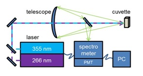
Figure 1: Simplified schematic view of the experimental setup.

All computations as described in the following part were executed with RStudio 1.1.442 using R 3.4.4 and in detail the caret package, which provides the utilization of over 200 models for classification and regression training [10-12].

First of all, those channels were eliminated which contain no or misleading information: the lower regions beyond both excitation wavelengths and the range of possible Raman peaks whose intensity could influence the scaling process and might lead to misclassifications caused by the presence of different solvents. Due to comparability reasons of different measurements the data were scaled by setting the minimum to 0 and the maximum to 1. The median spectrum of each substance is visualized by one plot per class in figure 2.

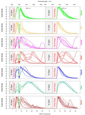Figure 2: Each plot shows the median of 100 signals for the belonging substances.

Finally, after modification the data contain information about the class to which they belong to and the normalized signal intensities from 47 features (27 for 266 nm excitation and 20 for 355 nm excitation). This dataset was passed to the model generation process where cross-validation and boot strapping were additionally performed to verify and optimize the classification models [8]. Taking the median (or mean) of several spectra is an optional step to gain even better results in less runtime but is not necessary within this scope and only done for visualization.

A scatter plot of the data of two channels is displayed in figure 3, reduced to the median of five consecutive signals and colored by class for a clearer segmentation. Despite that, the clusters are overlapping and cannot be separated well from each other but the classification is based on using all of the present features.

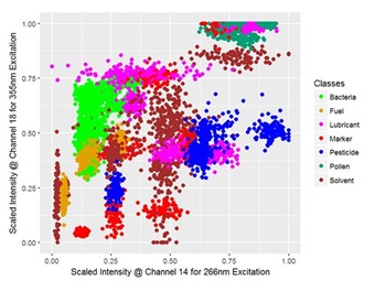Figure 3: Scatter plot for the scaled signal intensities of two features corresponding to the PMT-channel 14 and 18 which detect a 15 nm broad spectral region around 436.7 nm and 491.4 nm of the fluorescence signal excited by radiation with a wavelength of 266 nm and 355 nm, respectively; for visualization the dataset is reduced to the median of five consecutive spectra and colored by class.

In general, the aim of classification is the ability to predict the group to which an object belongs based on a set of features. Creating a reliable classification model consists of at least two steps, called training and test. In the training phase a part of the data is distinguished as good as possible by creating a predictive model for classification. In the test phase this model is validated with the remaining data to prevent a too specific discrimination by over fitted models. Here, the training set consists of 75 % of the data, resembled for a further reduction of overfitted [12].

Most of the algorithms provide a few variables which are adjusted during the training phase to gain best possible results. Every combination of those parameters is run separately and the final model can be chosen as the one with the highest accuracy, which is the ratio of the correctly predicted values to the total number of predictions. Within the method random forests many randomly generated decision trees classify the data [14]. The creation of these trees considers basic information of possible codomains of the thresholds and the sets are sampled among the given features. One variable is the amount of trees and another one is the number of sampled features which are randomly selected. The most frequent results of the different models are chosen as the best fit and used to build the final model by averaging their splitting thresholds. This can be processed several times with resampled training sets but within the present classification the tree structure did not change significantly after a few runs.

Instead of grouping the agents in seven classes it is also possible to identify the substances by their LIF spectra within the investigated dataset. Therefore, the modeling process is run again resulting in a new tree which has been trained with that intention. This second model might be used as well for a grouped prediction but it is rather overfitted and worse for that issue.

The information of the current measurement is gained from the excitation of different fluorophores utilizing laser pulses with two different excitation wavelengths. When the modeling process is run separately with each half of the data and additionally with the paired dataset it can be shown that this is an improvement. The results are summarized in a confusion matrix where the predictions are compared with the reference values.

The predictions are listed in table 2 showing that the utilization of a single excitation wavelength provides enough information to distinguish the classes (99.4 resp. 87.4 %). However using the complete dataset leads to even better results (99.9 %). If the substances are not divided in groups and ought to be discriminated precisely, the effect is more obvious. The single substances can be identified using both spectra with an accuracy of 94.1 % instead of 87.8 % resp. 74.5 % if only one of them is used. Even the very similar spectra of bacteria can be separated as shown in [1].

REFERENCES

- Gebert F, Kraus M, Fellner L, Arne W, Pargmann C, et al. (2018) Novel standoff detection system for the classification of chemical and biological hazardous substances combining temporal and spectral laser induced fluorescence techniques. 1st Scientific International Conference on CBRNe - SICC 2017, Rome, Italy.
- Kraus M, Fellner L, Gebert F, Grünewald K, Pargmann C, et al. (2017) Comparison of Classification methods for Spectral Data of Laser Induced Fluorescence. 1st Scientific International Conference on CBRNe - SICC 2017, Rome, Italy.
- Fischbach T, Duschek F, Hausmann A, Pargmann C, Aleksejev V, et al. (2015) Standoff detection and classification procedure for bioorganic compounds by hyperspectral laser-induced fluorescence. Chemical, Biological, Radiological, Nuclear, and Explosives (CBRNE) Sensing XVI, SPIE, USA. 9455: 9.
- Gaudio P, Gelfusa M, Murari A, Pizzoferrato R, Carestia M, et al. (2017) Application of optical techniques to detect chemical and biological agents. Defence S&T Technical Bulletin 10: 1-13.
- Buteau S, Ho J, Lahaie P, Rowsell S, Simard JR, et al. (2010) Laser based standoff detection of biological agents.
- Hay KG, Norberg O, Normand E, Önnerud H, Black P (2017) Development of an open-path gas analyser for plume detection in security applications. Advanced Optical Technologies 6: 67-73.
- Sun J, Ding J, Liu N, Yang G, Li J (2018) Detection of multiple chemicals based on external cavity quantum cascade laser spectroscopy. Spectrochim Acta A Mol Biomol Spectrosc 191: 532-538.
- Lantz B (2015) Machine Learning with R (2ndedn). Packt Publishing, Birmingham, UK.
- Duschek F, Fellner L, Gebert F, Grünewald K, Köhntopp A, et al. (2017) Standoff Detection and Classification of Bacteria by Multispectral Laser-Induced Fluorescence. Advanced Optical Technologies 6: 75-83.
- RStudio (2018) RStudio: Integrated Development Environment for R. RStudio, Boston, Massachusetts, USA.
- R Development Core Team (2016) R: A Language and Environment for Statistical Computing. R Foundation for Statistical Computing, Vienna, Austria.
- Kuhn M (2017) caret: Classification and Regression Training. ASCL, USA.
- Kuhn M, Johnson K (2013) Applied Predictive Modeling. Springer, New York, USA. Pg no: 600.
- Ho TK (1995) Random decision forests: ICDAR '95 Proceedings of the Third International Conference on Document Analysis and Recognition (Vol1). IEEE, Washington, New Jersey, USA. Pg no: 278.
- Fellner L, Gebert F, Walter A, Grünewald K, Duschek F (2017) Fluorescence Spectra of a Bacterial Population During Different Growth Phases. 1st Scientific International Conference on CBRNE, University of Rome Tor Vergata, Rom, Italy.
Citation: Kraus M, Fellner L, Gebert F, Pargmann C, Walter A, et al. (2018) Classification of Substances Combining Standoff Laser Induced Fluorescence and Machine Learning. J Light Laser Curr Trends 1: 003.
Copyright: © 2018 Marian Kraus, et al. This is an open-access article distributed under the terms of the Creative Commons Attribution License, which permits unrestricted use, distribution, and reproduction in any medium, provided the original author and source are credited.