Modelling Growth and Body Composition: A Comparative Analysis of Seven Commercially-Farmed Fish Species

Production of aquatic animals in 2020 reached a total of 178 million tonnes, in which 313 species of finfish were produced [1]. This suggests that there is significantly diversity among fish species produced, encompassing various aspects such as physiology, morphology, metabolism, ecology, and behaviour. Consequently, this heterogeneity presents challenges when it comes to, for instance, developing nutritional or growth models for every newly proposed species intended for commercial production, since the research required for each additional species incurs both time and costs. In this context, an important consideration is the generalizability of research findings: can the knowledge gained from studying one species be extended to other closely related species? For example, if a nutritional or growth model is validated for one species, can it reasonably be applied to a similar species? Evaluating generalizability helps determine the broader applicability of research findings. This leads to the transferability of knowledge: how can the knowledge obtained from studying one species be effectively employed to enhance the understanding of other species? By transferring knowledge, it is possible to contribute to practical advances in commercial production, conservation and resource management. Thus, the study of the similarity relationships between species through the use of objective criteria, such as, genetic [2-5], ecological [6, 7,8] or metabolic/nutritional [9-13] can assist in the development of nutritional models for farmed fish species. Through such modelling methodologies, it is possible to answer a range of technical and practical questions related to different production aspects, such as, nutritional requirements, optimal feed formulation, optimal feeding/rearing practices, expected growth performance, environmental impact of rearing activities, among others. 

In particular, body composition and/or nutrient/energy budget models can be used as objective criteria to explore the similarity relationships between species. To do so, species-specific models are calibrated and then compared either in terms of parametrization (for models with the same structure) or in terms of their predictions, with the assumption that the distances/similarities between species-specific models reflect the distances/similarities between the underlying species. The usual approach described in the literature to predict the body composition of fish is the use of isometric (a × body weight) or allometric  (a × body weight^b) models [14].The difference between isometric and allometric models is that the former assumes that the absolute content of each fish body component is proportional to body weight, whereas the latter assumes a non-proportional relationship between the content of each component and fish body weight. In nutrition studies, it is typically not feasible to conduct comprehensive evaluations of each parameter related to body composition due to the considerable time and effort required for data analysis. As a result, researchers usually make certain assumptions, such as “protein and/or ash follows an isometric pattern in fish” [15-19], often based on limited information or arbitrary/undeclared criteria, without considering the available evidence from other fish species. However, these assumptions may not always be accurate, particularly when assessing body composition in dynamic terms. Unfortunately, the lack of extensive comparisons between species hinders the establishment of global patterns and the ability to make conclusive statements about the effectiveness of these models in different contexts. Therefore, it is necessary to assess the relative merits of isometric vs. allometric models for each component to ensure a more accurate understanding of body composition and its relationship to nutrition in diverse fish species. 

To estimate fish growth accurately, models that consider the most important biological and physiological aspects of fish are often used, such as nutrient-based models, in which the fundamentals of energy and nutrient partitioning are considered. The energy-protein flux (EP) model, in particular, in addition to fish weight and temperature, considers both energy and protein intake to predict growth, while also estimating the body composition of fish based on protein retention equations [20]. The model explicitly assumes that energy requirements comprehend the energy for maintenance and growth [21], where maintenance metabolic expenditure (protein and energy losses) can be defined by exponents that determine the change in metabolic rate as a function of body weight [22]. However, there is a disagreement between authors regarding the definition of metabolic body weight exponents. Some authors advocate that an exponent of 0.75 can be used for several fish species [12,23,24], while others recommend the use of species-specific exponents [22,25,26]. Furthermore, while some authors suggest an exponent of 0.80 for energy and 0.70 for protein [13,21,26-28], others argue that, for some species, the same exponent should be used for both energy and protein [29,30]. Therefore, it is unclear whether one should assume the same exponents regardless of fish species or whether there are some similarities across a group of species that would justify using the same exponents and, ultimately, whether they should be different for energy and protein. 

In this work, seven commercial fish species that included Atlantic salmon (Salmo salar), gilthead seabream (Sparus aurata), European seabass (Dicentrarchus labrax), Nile tilapia (Oreochromis niloticus), rainbow trout (Oncorhynchus mykiss), turbot (Scophthalmus maximus) and Senegalese sole (Solea senegalensis), were compared on the basis of their body composition and growth performance characteristics. The goal was to assess certain assumptions and hypotheses present in the literature, such as whether isometric or allometric models should be used to describe body composition, the application of "universal" or species-specific metabolic body weight exponents, the use of constant or non-constant protein/energy efficiency ratios, and the assumption of compositional and metabolic similarity between species with similar genetic, morphological, ecological and physiological traits.

Comparison of body composition models

• Data collection 

Data on whole-body composition and weight were collected from the literature for seven species (Atlantic salmon, gilthead seabream, European seabass, Nile tilapia, rainbow trout, turbot and Senegalese sole) as shown in (Table 1) (see Appendix 1A for data sources). Data expressed on a dry matter basis were converted to a wet weight basis, according to [15] recommendation. Data were collected only from studies in which the whole fish content was determined according to the standard analytical methods of the Association of Official Analytical Chemists (AOAC). Carbohydrates are usually unreported, as they represent less than 0.14% of fish [31] and thus left out of this analysis. Each dataset was standardized to contain details about growth, body composition,

Feed Conversion Ratio (FCR), water temperature, and dietary properties.

Table 1: Overall data used for species comparison in terms of body weight and whole-body composition.

Model calibration and comparison

Body composition parameters between species were compared based on a set of estimates obtained from two different models (isometric and allometric), both calibrated with three different calibration methods (least squares linear regression, Huber loss linear regression and quantile regression). Additionally, within this process, to assessed how different data sources affected parameter estimates, Leave-One-Out (LOO) resampling or jackknife resampling [32] was performed. This procedure provided a measure of the variability of parameter estimates while considering the diverse datasets employed for model calibration. 

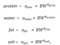
The equations and analysed parameters used in the isometric model were the following:

protein  =  a_prot   ×  BW

water  =   a_water ×  BW

fat  =   a_fat    ×  BW

ash =   a_ash   ×  BW 

where a gives information about the relative content of each component (assumes proportionality with body weight). 

In the allometric model, the following equations and analysed parameters were used:

where a gives information about the relative content of each component at a reference weight and b represents the effect of body weight on each component (assumes non-proportionality with body weight). 

For species displaying an isometric relationship between components and fish size, it is expect that the b parameter (i.e., body weight exponent) estimates for all components to be close to 1 (i.e., their logarithm to be close to zero). Thus, for each species, a (multiplicative) “distance from isometry” was calculated using Euclidian distance, as:

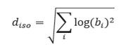where the sum is performed over the square of the logarithm of the body weight exponents of protein, water, fat and ash components. This distance is zero only when the species displays perfect isometry. Using the calculated distance, an “isometry index” was obtained in order to evaluate which species display a more stable body composition as they grow:

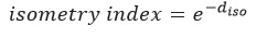This index is equal to 1 for species displaying perfect isometry (perfectly stable composition throughout the body weight range), and the lower value, the farther the species is from isometry (body composition changes throughout the body weight range).

The similarity relationships between species in terms of body composition were evaluated through Principal Component Analysis (PCA), by plotting their respective parameter estimates along the first two principal components. Furthermore, species were compared based on the predictions of isometric and allometric models for their body composition components. This comparison was made through visual observation of line plots. Additionally, the results of both models were assessed for agreement by comparing them through scatterplots. All analyses were performed using R version 4.1.2 [33], where the lm function from the ‘stats' package [33] was used for least squares regression, the rlm function from the ‘MASS’ package [34] was used for Huber loss linear regression (robust regression), and the rq function from the ‘quantreg’ package [35] was used for quantile regression.

Comparison of energy/nutrient budget models

• Data collection 

Data on growth trials covering a wide range of rearing conditions and feed properties were collected from the literature for the selected species (see Table 2 and Appendix 1B for an overview of the collected data). Senegalese sole growth data were too heterogeneous and patchy (with regards to the joint “body weight and temperature” distribution) and, thus, were left out of the growth comparison to avoid effect confounding and a biased analysis. All datasets were converted into a standard format, where information on the growth, body composition, Fed Conversion Ratio (FCR), water temperature, feed intake and diet properties are stored on a daily resolution basis. Missing data were handled by using default values (e.g., apparent digestibility coefficients) or by applying interpolation methods (e.g., daily feed intake was estimated based on FCR and growth, when not explicitly reported in the data source).

Table 2: Overall data used for species comparison in terms of growth parameters.

ww- wet weight;

DP/DE – digestible protein and energy ratio

Model calibration and comparison 

For each species, an Energy-Protein flux (EP) model was developed in which, for both energy and protein, a balance between a feed-dependent gain and a feed-independent loss was calculated:

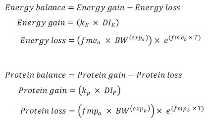Where:

The feed-dependent gain depends on an efficiency coefficient (k), and the feed-independent loss in turn depends on the effect of the body weight and temperature. The models were calibrated based on different assumptions, which resulted in four different calibration methods (see Table 3).  For a better interpretation of the results of the effect of temperature on fasting maintenance costs, the fme_b and fmp_b parameters were converted and reported as

Q10 (temperature coefficient) values (i.e.,

Table 3: Definition of growth model and calibration methods used for species comparison.

Due to the occasional presence of extreme outlying parameter estimates for some of the leave-one-out folds, which prevents a meaningful PCA analysis, a filtering step was added using a simple univariate rule for outlier detection and removal (|z-score| > 3). This rule is based on the property of the standard Gaussian distribution that 99.7% of its values lie between -3 and 3, thus any z-score greater than +3 or less than -3 can be considered as outlier if assuming the parameter distributions to be approximately Gaussian and the number of observations relatively low [36,37]. 

The similarity relationships between species in terms of protein/energy budgets were initially evaluated through PCA analysis, by plotting their respective parameter estimates along the first two principal components. Additionally, the predictions from models calibrated with different methods were assessed through scatter plots to determine if the predictions agreed or not, when fixed universal or estimated parameters were used in the calibration process. All analyses were performed using the regression functions mentioned in section 2.1.2 Model calibration and comparison.

• General similarities between species body composition and growth parameters 

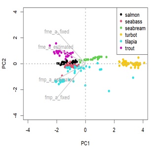
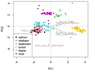
The similarity between species in terms of model parameters was evaluated using a PCA analysis (Figure 1). In this analysis, it can be assumed that the distances between points for each species reflect the differences in parameter estimates (e.g., when the points are closer, it indicates that the parameter estimates are more similar) Results suggest that similarities within salmonids are the strongest, consistent across parameters and thus clearer in both PCA projections (Figures 1a&1b). Despite having some differences in growth (Figure 1b&Appendix 2), seabream and seabass show strong similarities in terms of body composition parameters (Figure 1a). Flatfish species, however, do not group as clearly. In fact, turbot and sole have distinct body composition parameters (Figure 1a). 

Appendix 2

Here several PCA analyses based on the different parameters of the growth models are given. These analyses provide insight into which parameters are similar across species, and whether they remain consistent when body weight exponents are either universal or estimated.

Appendix 2a: Principal component analysis (PCA) displaying species distance in terms of maintenance costs parameters.

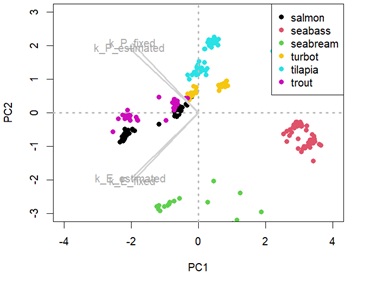
Appendix 2b: Principal component analysis (PCA) showing species distance in terms of retention efficiency parameters.

Appendix 2C: Principal component analysis (PCA) showing species distance considering the metabolic body weight and temperature effect. 

Overall, PCA analysis suggests that water and fat parameters are negatively correlated, and that isometry index is more related with these than with the other components (Figure 1a).

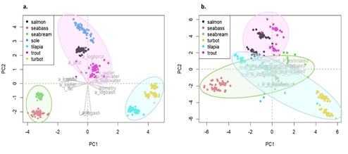Figure 1a: Principal component analysis (PCA) with estimates of parameter a for each component according to an isometric and an allometric model for each species, parameter b and with the isometry index. ai prefix correspond to parameter a estimated by isometric model; aa and b prefix corresponds to parameter a or b estimated by allometric model. Circles with different colour indicates the species clusters: green circle seabream and seabass species (seabream and seabass); pink circle salmonids (salmon and trout) and sole; blue circle tilapia and turbot. b. Principal Component Analysis (PCA) displaying the overall distance between species, considering the estimates or the use of fixed universal parameters to predict growth. Circles with different colours indicate the species clusters. The figure shows an overlapping of species clusters and some distance between species within some cluster, due to differences in parameters estimations.

Body composition similarities

(Figure 2) shows estimates for the relative content of each body component and how they are affected by body weight, for each species, based on the species-specific allometric models (see Appendix 3 for details). Overall, the differences between species in terms of whole-body composition become more pronounced as they grow. This implies that the body composition of small fish (e.g., approximately 1 g) may not be species-dependent (or only weakly so). For instance, when comparing species at a reference body weight of 1 g, fat to vary between 2.5 – 7.5 %, whereas when comparing species at reference body weight of 1 kg, the variations are between 5 – 30 % approximately. Ranking fish species in terms of relative fat content at a reference weight of 1kg, seabass and seabream are the fattest species with approximately 20%, followed by salmonids (salmon and rainbow trout) with about 15%, sole with 10%, and tilapia and turbot as the leanest species with approximately 5% fat relative content.  For water, the opposite pattern is observed: turbot is the species with highest water relative content (» 75% of its body weight), followed by tilapia and sole (» 70%), salmonids (» 65%), and seabass and seabream with the lowest values (» 60% water). In terms of protein, sole is the species with the highest relative content (» 20%), followed by salmon and seabream (» 18%), and then seabass, rainbow trout, tilapia and turbot (less than 18% of protein). The ash relative content vary greatly even within species and is therefore more difficult to analyse. However, it tilapia, turbot, seabass and seabream are the species with the highest ash relative content, while salmonids and sole are the ones with the lowest values. 

In terms of how body components are affected by body weight (parameter b), relative water and fat content show high variation, but with clear patterns: water tends to decrease with body weight, whereas fat tends to increase (see Figure 2). Despite the variation, the water slopes seem to be constant and generally negative (b_water < 1) for all species (see Appendix 3C for details). For fat, slopes are positive (b_fat > 1) and variable for all species, being higher for seabream and seabass (highest accumulation of fat as they grow) and lower for tilapia and turbot (lowest accumulation of fat as they grow) (see Appendix 3B for details). Protein increase as the body weight increases, except for seabass, where the protein content in relative terms seems to be less affected by the body weight, and thus more constant. In fact, the slope tends to be close to zero and b_prot much closer to 1 for seabass, when compared with other species (see Appendix 3A for details). In turn, the effect of body weight on relative ash levels does not present a clear and consistent pattern across species. The relationship between ash relative content and body weight is very variable between and within species (sometimes b_ash is above 1, other times below 1), making it unclear whether there is a consistent effect of body weight on ash relative content (see Appendix 3D for details). Moreover, comparing the isometry index between species (Figure 3), tilapia and turbot seem to be the species closest to isometry, meaning that the effect of the body weight on body components is less strong. In fact, tilapia and turbot parameters are in general closer to 1 (isometry) when compared to other species in this study (see Appendix 3). In contrast, seabass and seabream seem to be the ones furthest from isometry, which is consistent with what is shown in (Figure 2), where the effects of body weight on body components are generally noticeable. 

Regarding the parameter a estimates, there was a general agreement between the isometric and allometric model for each body component of the different species (Figure 4). However, in the specific case of protein, the a_prot estimates between the two types of models seem to display lower correlation. Despite this, it is possible to see the same pattern in both isometric and allometric predictions: tilapia, turbot and rainbow trout seem to have lower a_prot values than the other species (i.e., lower protein relative content). In terms of fat, the a_fat parameter is higher for seabass/seabream and lower for turbot. In turn, the aash parameter is to be lower for salmonids and sole, and higher for the other species. 

Consistent with the PCA analysis, there is a clear negative correlation between fat and water relative content (F-test, p-value < 0.001), according to both allometric and isometric models (Figure 5). Between water and the other two components (protein and ash) there is no such clear pattern. Although a statistically significant negative correlation is present for the isometric model (F-test, p-value < 0.001), these effects are not as clear for the allometric model and are no longer significant for the ash component (F-test, p-value > 0.05). 

In general, estimates of the b parameter were also consistent between calibration methods (see Appendix 3), except for b_ash.

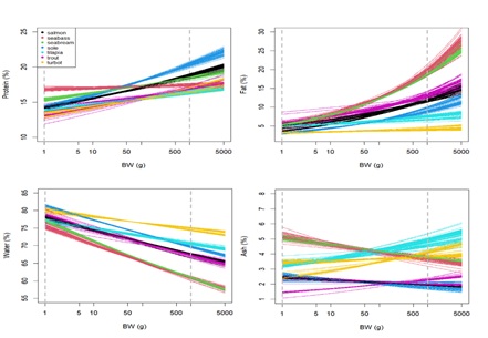
Figure 2 : Line plots showing predictions of body composition components as a function of body weight. Solid lines represent the predictions obtained for each model (calibrated on a LOO sample). Different colour lines denote different species. Dashed grey lines indicates body weight = 1 g and body weight = 5000g.

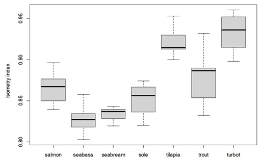Figure 3 : Boxplot of the isometry index, demonstrating how each species body composition is affected by body weight (closer to value 1, means that the overall species body composition is not dependent/affected by body weight). The middle line in the box is the median. The box, divided into two parts shows the first quartile and the third quartile (Q1, at the bottom of the box, represents the lowest 25% of the data and the Q3, the upper part of the box, represents the highest 25% of the data). The whiskers show the minimum and maximum values within the data that are not considered outliers. Outliers are shown as individual points beyond the whiskers.

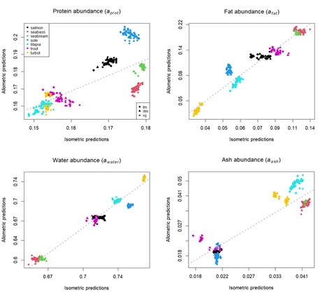Figure 4 : Scatterplots showing allometric and isometric estimates for parameter a, for each body composition component. Points represent parameter a estimates according to each calibration method. Different colours indicate different species. Grey dashed line is the linear regression between allometric and isometric estimates.

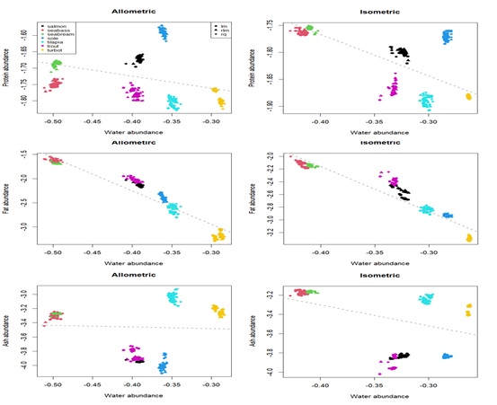Figure 5 : Scatterplots showing the relation between water and other body composition components, according to allometric and isometric models. Points represent parameter a estimates according to each calibration method. Different colour point denotes each species. Grey dashed line is the linear regression between components.

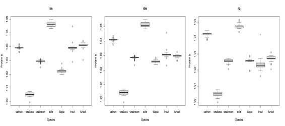Appendix 3A: Box plot displaying parameter b estimates for protein with different types of regressions for the compared species. lm = least squares linear regression; rlm = Huber loss linear regression; rq = quantile regression. The middle line in the box is the median. The box, divided into two parts shows the first quartile and the third quartile (Q1, at the bottom of the box, represents the lowest 25% of the data and the Q3, the upper part of the box, represents the highest 25% of the data). The whiskers show the minimum and maximum values within the data that are not considered outliers. Outliers are shown as individual points beyond the whiskers.

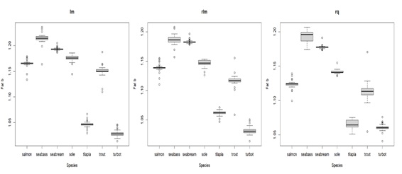Appendix 3B: Box plot displaying parameter b estimates for fat with different types of regressions for the compared species. lm = least squares linear regression; rlm = Huber loss linear regression; rq = quantile regression. The middle line in the box is the median. The box, divided into two parts shows the first quartile and the third quartile (Q1, at the bottom of the box, represents the lowest 25% of the data and the Q3, the upper part of the box, represents the highest 25% of the data). The whiskers show the minimum and maximum values within the data that are not considered outliers. Outliers are shown as individual points beyond the whiskers.

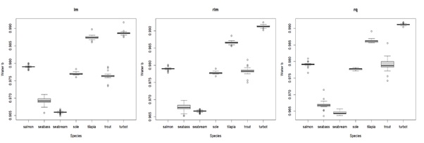Appendix 3C: Box plot displaying parameter b estimates for water with different types of regressions for the compared species. lm = least squares linear regression; rlm = Huber loss linear regression; rq = quantile regression. The middle line in the box is the median. The box, divided into two parts shows the first quartile and the third quartile (Q1, at the bottom of the box, represents the lowest 25% of the data and the Q3, the upper part of the box, represents the highest 25% of the data). The whiskers show the minimum and maximum values within the data that are not considered outliers. Outliers are shown as individual points beyond the whiskers.

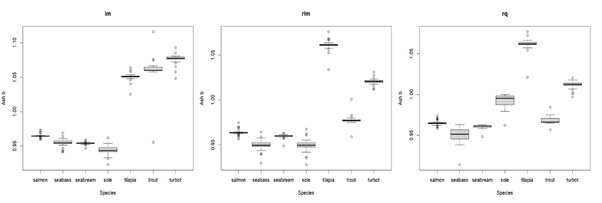 Appendix 3D: Box plot displaying parameter b estimates for ash with different types of regressions for the compared species. lm = least squares linear regression; rlm = Huber loss linear regression; rq = quantile regression. The middle line in the box is the median. The box, divided into two parts shows the first quartile and the third quartile (Q1, at the bottom of the box, represents the lowest 25% of the data and the Q3, the upper part of the box, represents the highest 25% of the data). The whiskers show the minimum and maximum values within the data that are not considered outliers. Outliers are shown as individual points beyond the whiskers.

Energy/nutrient budget similarities

• Metabolic body weight exponent 

Overall, the estimated metabolic body weight exponents for energy (exp_e) and protein (exp_p) were not far from what is reported in the literature (0.80 and 0.70 for energy and protein, respectively (Clarke & Johnston, 1999; Lupatsch et al., 2003ab)). The estimate ranges for exp_e were slightly different between species: salmon 0.82 – 0.87; seabass 0.71 – 0.89; seabream 0.51 – 0.72; tilapia 0.69 – 0.85; rainbow trout 0.62 – 0.80; turbot 0.70 – 0.85 (Figure 6). For some species, such as salmon and seabream, the estimated range do not include the standard value of 0.80. Moreover, for tilapia and trout, most estimates were below 0.80. Seabass and turbot were the only species for which the putative universal exponent (0.80) was found within the estimated range for the parameter exp_e. 

For protein, exp_p estimates also seem to be quite different between species: salmon 0.77 – 0.83; seabass 0.78 – 0.97; seabream 0.54 – 0.88; tilapia 0.73 – 0.85; rainbow trout 0.71 – 0.78; turbot 0.61 – 0.74 (Figure 6). In this case, the standard value of 0.70 is not found within the estimated ranges for salmon, seabass, tilapia and trout. Seabream and turbot are the only species for which the estimated range for exp_p include the assumed universal value of 0.70.

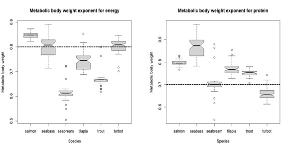Figure 6: Boxplot showing the estimates of metabolic body weight exponents for energy (exp_e ) on the left, and for protein (exp_p ) on the right, according to each species. The middle line in the box is the median. The box, divided into two parts shows the first quartile and the third quartile (Q1, at the bottom of the box, represents the lowest 25% of the data and the Q3, the upper part of the box, represents the highest 25% of the data). The whiskers show the minimum and maximum values within the data that are not considered outliers. Outliers are shown as individual points beyond the whiskers. The boxplot notches indicate an approximate 95% confidence interval for the median. Dashed line represents the so-called universal value for metabolic body weight exponent for energy (left) and protein (right).

• Energy fasting maintenance 

When converting the estimates of the fme_b parameter (which gives information on the effect of temperature on the maintenance costs for energy) to Q10 values, almost all species exhibited values ranging between 1 and 2, with the exception of turbot (Figure 7). Turbot is the species where fasting maintenance costs for energy are most affected by temperature, exhibiting the highest Q10 estimates (approximately 3.5). In turn, rainbow trout appears to be the species in which the energy costs are less influenced by temperature, displaying the lowest Q10 values estimates (approximately 1). The fme_b estimates do not seem to be affected by the calibration methods used (see Appendix 4A for more details).

The estimates for relative energy fasting maintenance costs generally remain consistent when using universal or estimated body weight exponents (see Appendix 3B for details). Species demonstrate differences in relative energy fasting maintenance costs, with turbot having the lowest costs under reference body weight and temperature conditions, followed by tilapia, seabass, and seabream (see Appendix 4B). Tilapia seem to be particularly close to seabass. Salmon and rainbow trout, on the other hand, exhibit higher fasting maintenance costs in comparison (fme_a).

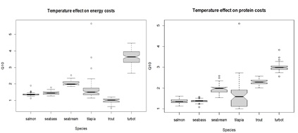Figure 7: Box plots displaying Q10 value estimates for temperature effects on energy (left) and protein (right) fasting maintenance costs. The middle line in the box is the median. The box, divided into two parts shows the first quartile and the third quartile (Q1, at the bottom of the box, represents the lowest 25% of the data and the Q3, the upper part of the box, represents the highest 25% of the data). The whiskers show the minimum and maximum values within the data that are not considered outliers. Outliers are shown as individual points beyond the whiskers. The boxplot notches indicate an approximate 95% confidence interval for the median.

Appendix 4

This appendix contains the results of a comparison made between the estimates of the different parameters of the growth models, using fixed universal and estimated parameters, and with different calibration methods. The scatterplots below are useful to understand which species tend to have higher or lower parameters and how similar or different they are between each other.

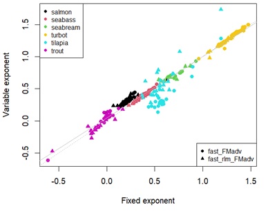Appendix 4A: Scatterplot showing estimates effect of temperature on fasting maintenance costs for energy using fixed universal or estimated parameters. Different points represent the type of linear regression used. Different colour points represent each species. Grey dashed line denotes y=x. Solid grey line represents the linear regression between estimates.

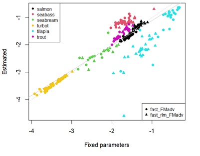
Appendix 4B: Scatterplot showing estimates of fasting maintenance costs for energy using fixed universal or estimated parameters in log scale. Different points represent the type of linear regression used. Different colour points represent each species. Grey dashed line denotes y=x. Solid grey line represents the linear regression between estimates.

• Protein fasting maintenance

When converting the estimates of the fmp_b parameter into Q10 values, most species exhibited values ranging between 1 and 2, apart from turbot and rainbow trout, where the estimated Q10 values were > 2. Turbot and rainbow trout seem to be the species where the fasting maintenance costs for protein are more affected by temperature (see Appendix 4C). Species such as tilapia, salmon and seabass seem to be those where the relative fasting maintenance costs for protein are least affected by temperature, followed by seabream (see Appendix 4C).

Tilapia is the species with higher relative fasting maintenance costs for protein under reference conditions (fmp_a) (see Appendix 4D). Other species like salmon, seabass and rainbow trout seem to have lower relative fasting maintenance costs for protein when compared with tilapia. 

In general, the estimates for fmp_b and fmp_a remain consistent regardless of the calibration methods employed, except for tilapia, where some differences are observed between the least squares linear regression and Huber loss linear regression approaches (i.e., lm and rlm, respectively) (see Appendix 4C&4D for more details). 

Appendix 4C: Scatterplot showing estimates of temperature effect on fasting maintenance costs for protein using fixed universal or estimated parameters. Different points represent the type of linear regression used. Different colour points represent each species. Grey dashed line denotes y=x. Solid grey line represents the linear regression between estimates.

Appendix 4D: Scatterplot showing estimates of fasting maintenance costs for protein using fixed universal or estimated parameters in log scale. Different points represent the type of linear regression used. Different colour points represent each species. Grey dashed line denotes y=x. Solid grey line represents the linear regression between estimates.

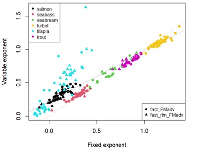
Appendix 4E: Scatterplot showing estimates of energy retention efficiency using fixed universal or estimated parameters. Different points represent the type of linear regression used. Different colour points represent each species. Grey dashed line denotes y=x. Solid grey line represents the linear regression between estimates.

• Retention efficiency 

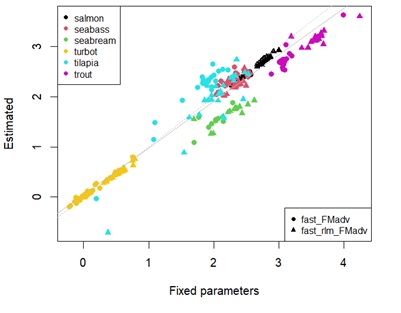
(Figure 8) shows the estimated values for the energy retention efficiency coefficients. In terms of energy retention, species can be separated into two groups: species with coefficients between 0.45 and 0.50 (e.g., salmon, seabream and trout) and species with coefficients between 0.50 and 0.60 (e.g., seabass, tilapia and turbot). When considering protein retention coefficients, salmon, tilapia, trout, and turbot exhibited higher values (0.55 – 0.65), while seabass and seabream displayed lower values (0.40 – 0.50). 

Estimates for energy and protein retention efficiency are insensitive to the use of either universal or estimated metabolic body weight exponents, but there are some differences in terms of the type of linear regression used (e.g., lm and rlm) (see Appendix 4F for details). 

Overall, salmonid species (salmon and rainbow trout) can be grouped together according to their highest retention efficiency for protein and energy, as illustrated previously in the PCA analysis (Figure 1b). Seabream and seabass present differences in energy retention coefficients (see Appendix 4E for details). In turn, tilapia and turbot display closer estimates for both energy and protein retention efficiencies.

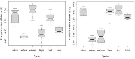Figure 8: Box plot showing the estimates range for energy (left) and protein (right) retention efficiency. The middle line in the box is the median. The box, divided into two parts shows the first quartile and the third quartile (Q1, at the bottom of the box, represents the lowest 25% of the data and the Q3, the upper part of the box, represents the highest 25% of the data). The whiskers show the minimum and maximum values within the data that are not considered outliers. Outliers are shown as individual points beyond the whiskers. The boxplot notches indicate an approximate 95% confidence interval for the median.

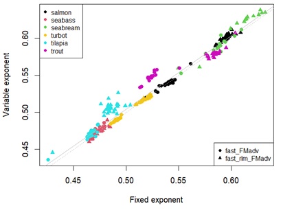
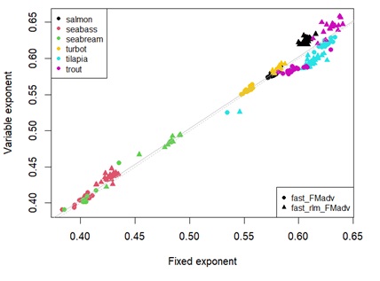Appendix 4F: Scatterplot showing estimates of protein retention efficiency using fixed universal or estimated parameters. Different points represent the type of linear regression used. Different colour points represent each species. Grey dashed line denotes y=x. Solid grey line represents the linear regression between estimates.

 General similarities between species body composition and growth parameters 

It is usually assumed that there should be similarity in terms of body composition and growth between species with similar phylogeny, morphology, ecology and/or physiology. In this study, species were grouped based on similarities in body composition and growth models. In particular: 1) salmonids, with strong and consistent similarities across parameters; and 2) Seabream and seabass with body composition similarities but differences in growth parameters. Flatfish species, in turn, did not group as clearly. 

The body composition of the fish is determined by the capacity of species to retain the different macronutrients. Here similarities were found between species in both body composition and growth analyses. Furthermore, the distances in space between species in relation to body composition parameters are, in some cases, similar to those found for the parameters of the growth model. While salmonids are generally close in both analyses, there is not such a clear homogeneity between seabream and seabass and flatfish species. The distance between tilapia and turbot was also different in the two analyses. Tilapia showed similar body composition to turbot, although these similarities were not reflected in the analysis of growth parameters, which may be related to differences in feeding habits (carnivorous vs. omnivorous) and metabolism.  

Body composition similarities 

When analysing the similarities in terms of body composition among different species, it was noticeable that species exhibited a higher degree of similarity at very low body weights. Results suggest that, as they grow, fish species tend to diverge in terms of body composition. Seabream and seabass fish species have higher relative fat content than salmonids, when measured at similar body weights. Moreover, salmon tends to have higher protein and lower fat relative content than rainbow trout, as reported by previous authors [38,39]. It is important to note, however, that the distribution of data collected for each species varies significantly. For example, for salmon, the database mostly contains information on fish weighing around 51.8 g (median), while for seabass and seabream, the data mostly corresponds to fish weighing approximately 90 g (median). Additionally, the data for salmon covers fish weighing up to 4950 g, while it does not exceed 1000 g for seabream and seabass. Thus, despite these results, some caution should be taken when extrapolating to values outside the range of those used to perform the regression. In flatfish species (i.e., sole and turbot), this divergence may be related to differences in their trophic level (sole 3.2 vs. turbot 4.4) [40], metabolism or to other factors that may be determined by the different geographic distributions of the two species, such as temperature or depth [41]. Seabream and seabass are the species where the fat relative content is most affected by body weight (i.e., furthest from isometry), which implies that these species tend to have more variations of fat levels throughout their growth. In turn, tilapia and turbot seem to be the species where the body composition is less affected by body weight (i.e., closest to isometry). In fact, Raposo et al. [42] reported that, though the body composition of Nile tilapia seems to be allometric, the body weight exponent (b parameter) is close to 1 and that, in some cases, it may be reasonable to use isometric models or intermediate models between a purely isometric and allometric models (e.g., ensemble models) to predict Nile tilapia body composition. 

The estimates for ash, in this study, turn out to be very variable between and within species, especially for the b parameter (b_ash), making it difficult to conclude if there are some differences between compared species, and whether b_ash is generally different from (i.e., above or below) 1. Generally, ash is the less abundant body composition component in fish and is thus difficult to be determined with precision, due to sample homogenization and manipulation (e.g., if fish samples are not well homogenized, some may contain more scales or bones, which may affect the measurement of ash content by analytical methods). Thus, this may in part explain the variability for b_ash estimates.  Furthermore, the variability in b_ash estimates may also be related to the Leave-One-Out (LOO) resample method used. This is because, when a source related to fish that are either too big or too small is excluded from the estimation, the estimation of the b parameter is performed without this information, leading to variable estimates.  Additionally, the use of the LOO resampling method, which involves using different datasets in each fold, significantly impacts the estimation of these specific parameters compared to others. Thus, when estimating exponents (e.g., b parameter or metabolic body weight exponent), the obtained estimates tend to be highly sensitive to the chosen dataset, contributing significantly to the general variability observed in the estimates. Overall, it seems that the general assumption of isometry for ash (b_ash = 1) is consistent with our results and probably will not significantly compromise the accuracy of predictions. 

Energy/nutrient budget similarities

• Metabolic body weight exponent 

Fish growth is a result of several metabolic processes that require energy and thus, may interactively affect metabolic scaling [43], However, there is a great controversy among authors regarding the exponent of metabolic body weight, which complicates the modelling of fish metabolism and growth. The primary point of contention lies in determining the appropriate and accurate value for the exponent that describes the scaling relationship between metabolic rate and body weight in fish. This controversy makes it difficult to establish a consensus or standardized approach for estimating metabolic rates in fish and understanding their energetics, growth and ecological interactions. In this study, results suggest that the metabolic body weight exponent is different for energy and protein, as reported in previous studies [21,25,27,28,44]. Moreover, both energy and protein metabolic body weight exponents may be species-specific, ranging from 0.51 to 0.89, challenging the concept of universal metabolic allometry [41,43,45-47]. The metabolic body weights for energy estimated in the present study are either within or near the ranges reported for the analysed species: salmon 0.82 – 0.87 vs. 0.85 – 1.06 reported by [48,49]; seabass 0.71 – 0.89 vs. 0.8 [50]; tilapia 0.69 – 0.85 vs. 0.75 and 0.8 reported by [24,30], respectively; rainbow trout 0.62 – 0.80 vs. 0.8 [27]; turbot 0.70 – 0.85 vs 0.7 [51]. However, for seabream a range of 0.51 – 0.72 was obtained, which does not include the value 0.80 reported by [13,48]. Although comparable data concerning the metabolic body weight for protein is scarce, some reference values exist in the literature for seabass, seabream, tilapia and rainbow trout. For seabass, the estimated metabolic exponent for protein ranges from 0.78 to 0.97, which does not include the value 0.70 reported by [50]; for seabream, it is between 0.54 and 0.88 vs. 0.70 [13,48]; for Nile tilapia 0.73 to 0.85 vs. 0.80, close to the value previously reported by Van Trung et al. [30]; for rainbow trout 0.71 to 0.78, similar to the 0.70 value reported by [27]. The variability of metabolic scaling values between species in this study may be related to taxonomy [12,43,46,52,53], physiological stages [52,54,55], ecological features [56], fish activity [11,41,46, 55,56], fish metabolism [9,38] Grisdale?Helland et al., [57,58], typical and maximum body mass [43,59], as stated in previous studies. 

• Energy and protein fasting maintenance 

Fish fasting maintenance costs are closely correlated with their size and temperature. It is therefore usual to evaluate the effect of temperature on fasting maintenance costs using the Q10 factor, as it allows to describe and quantify the influence of temperature on the kinetics of the maintenance process in fish. In this study, the Q10 values for energy and protein fasting maintenance costs were, in general, in agreement with what has been reported for teleost fish species [12,60,61]. However, when comparing the values between species, the Q10 values for the turbot were higher. Moreover, turbot seem to have lower maintenance costs energy and protein, when compared to other fish species. The difference in maintenance cost parameters for energy between turbot and the other species may be related to differences in swimming mode, which consequently relates to the fish body form [62]. Additionally, fish body form is often closely related to the specific habitats that fish inhabit [63-65]. Turbot is a benthic flatfish species that alternates its swimming form between a balistiform mode, which is used to swim slowly on the bottom, or anguilliform when it needs to swim faster [66]. Additionally, it is a sit-and-wait/slow forage [41,56,66]. Thus, it is a species with lower activity compared to pelagic (e.g., seabass and seabream) or benthopelagic species (e.g., salmon and rainbow trout), which are more active foragers and have different swimming modes. Turbot, therefore, has less metabolic expenditures compared to seabream, seabass, salmon and rainbow trout [41,56,66,67], which may partly explain the large differences in their fasting maintenance costs parameters for energy compared to other species. Regarding protein maintenance cost parameters, rainbow trout, salmon and seabass turn out to be similar. Others (e.g., seabream, tilapia and turbot) showed species-specific parameters, which may be reflected in different amino acid requirements between species [68,69]. 

• Energy and protein retention efficiency 

Marine fish live in an environment where the concentration of salts and minerals is higher than in freshwater, which can lead to differences in how they process dietary energy and protein [54,39]. Some studies have suggested that differences between fresh and marine water species, in addition to osmoregulation differences, may be in part due to variations in the types microorganisms in their digestive systems [35,70]. In the present study, seabream displayed higher energy retention efficiency than the other species, especially compared to seabass, which contradicts the similarity that Lupatsch et al. [26] reported between these two species. Furthermore, salmon presented higher energy retention efficiencies than rainbow trout as reported by Azevedo et al. [9,38]. Seabass and tilapia were the species with lower energy retention efficiency, but no characteristic between the two species was found to justify this similarity. In terms of protein retention efficiency, freshwater (i.e., Nile tilapia) and anadromous species (i.e., Atlantic salmon and rainbow trout) are more efficient than marine species (i.e., seabass and seabream). This is in line with  Tibaldi & Kaushik [69] previous report that seabream and seabass were less efficient at converting protein compared to salmonids. This may be at least partially attributed to the extensive history of breeding programs for salmonids (over 11 generations), while species like sea bass or sea bream have undergone fewer than nine generations of breeding, as noted by Chavanne et al. [71]. However, as reported by de Verdal et al. [70], enhancing feed efficiency in fish through selective breeding poses numerous challenges. It appears that the response to selection often remains inconclusive due to the limited genetic variation observed in traits associated with feed efficiency. While some authors reported that differences in digestibility may partly explain the variation in observed protein retention ability among species [31,72,73], our findings suggest that the discrepancy in protein retention between the studied freshwater, anadromous, and marine species may be primarily attributed to metabolic differences rather than digestibility. Furthermore, the efficient protein retention displayed by Nile tilapia, despite belonging to a lower trophic level (2) as an omnivorous species, could be attributed to its ability to utilize not only fat and protein, but also carbohydrates as an energy source [74,75]. By utilizing carbohydrates as an additional energy source, Nile tilapia can reduce the reliance on protein for energy production (i.e., protein sparing effect). This efficient allocation of protein helps in optimizing growth and overall energy utilization. Thus, it enables tilapia to allocate more protein towards muscle development and growth rather than using a larger proportion for energy production [74-77]. Although there is some controversy regarding the comparative protein retention efficiency of carnivorous and omnivorous fish species [10,78-84], it is clear that protein digestibility and retention rates vary depending on fish species, metabolism, diet composition, trophic level and other factors. Thus, it is difficult to make broad generalizations about carnivorous versus omnivorous fish and the same applies to freshwater versus marine fish. 

• Practical applications and insights from body composition and growth analysis in fish species

This work has several potential practical applications beyond contributing to the understanding of nutritional status and growth of commercially-relevant fish species. For instance, based on the data obtained from body composition analysis, it is possible to develop a software tool that can identify anomalies (i.e., gross errors) in the results obtained from the chemical analysis. This would be useful to determine if the body composition results from the chemical analysis are in the correct range or if there are any samples that present some anomaly, providing quality control measures that are essential in ensuring the accuracy and reliability of the data generated from this analysis. The intent is for this type of automated quality control analysis to become more widely adopted as practical, user-friendly tools for predicting body composition become available (Soares et al., 2023). A software tool like this can also help farmers to track the quality of their stock and make feed adjustments, if necessary, to assure fish health and growth. 

Since, in aquaculture, there is a large number of species being produced, having the ability to calibrate models (e.g., body composition and growth models) for new species with a limited number of samples can be useful when new species are proposed for production. This means that, if a farmer wanted to start farming a new species of fish, this method can be used to predict the growth patterns and body composition of the new species, helping to plan feeding and growth strategies. Furthermore, if two species have similar growth patterns, they could potentially be farmed together, thereby saving resources. One potential approach is to use the model to predict the samples for each identified species, and then utilize the prediction error to estimate the distance from each reference species. By using a suitable scheme (e.g., inverse distance weighting) to aggregate parameter or prediction estimates from the reference models, predictions for the new species can be obtained. This type of approach can enable the prediction of body composition or growth patterns for new species based on a set of reference species and potentially assist in the calibration of models for these new species with limited data availability (e.g., through the generation of synthetic data). Additionally, the information about the similarity between species in terms of body composition can be used to estimate the similarity in terms of growth between the same species or vice versa. An example of this type of approach is described in Appendix 5, which shows how body composition information could be used to predict the parametrization of growth models for different species.

Appendix 5

In this appendix, a practical example is given of how the obtained and processed information in this study can be used. Herein, the distance between species estimates, for both body composition and growth, were assumed to characterize the distance in similarity between species. Moreover, in growth comparison analysis, as stated previously, Senegalese sole was left out due to scarcity of data. However, it is suggested that it may be possible through the method of Partial Least Squares regression (PLS) to predict its growth similarity with other species, based on the data of body composition parameters (i.e., distance between sole and other species on body composition predictions). 

After using the PLS method for prediction of growth parameters based on body composition parameters, a PCA analysis was performed to evaluate the overall differences between true and the predicted general growth parameters of species [Appendix 5.A1(A)]. The results shown that in general, the EP parameter predictions obtained from the body composition parameters are close to the true values. Taking these estimates as accurate, Senegalese sole have some similarities with turbot. However, regarding the metabolic body weight for energy, Senegalese sole displays exponents closer to Nile tilapia, while the exponents for protein are more alike turbot and rainbow trout [Appendix 5A1(B)]. In terms of retention efficiency, sole have energy retention efficiency similar to the Atlantic salmon and protein retention efficiency similar to that of salmonids, Nile tilapia and turbot [Appendix 5.A1(C)]. 

This method allows us to get an estimate of the growth patterns of different species when data (e.g., growth trials) are scarce.

Appendix 5A1: Results obtained by using PLS method to predict the distance/similarity of Senegalese sole in relation to other species. Scatterplot (A) shows the PCA analysis of general growth parameters predictions of sole and other species. Scatterplots (B) e (C) shows the true and predicted metabolic body weight exponents for protein (mbw_exp_P) and energy (mbw_exp_E), and protein (k_P) and energy (k_E) efficiency, respectively. Open circles are the true values and full squares represent the estimates of each species.

The findings of this study indicate that, although some species may have some particularities in common (e.g., same family, geographical area, similar diets or body shapes), it does not mean that they are necessarily similar with regards to other aspects. In the particular case of the two salmonids studied, our analysis showed that they are indeed similar both in terms of body composition and growth. In turn, the Mediterranean species studied, seabream and seabass, while similar in terms of body composition, display some differences in growth parameters. Furthermore, while there is high similarity in terms of body composition among all species in their early juvenile stages, this similarity decreases as they grow. Additionally, the evaluation of growth parameters suggests that the metabolic body weight exponent is species-specific, contradicting the theory of a universal law for metabolic scaling. Differences in growth parameters between species can be related to their distinct retention efficiencies for energy and protein as well as to unique fasting maintenance costs, encompassing energy and protein requirements. The fasting maintenance costs are intricately linked to factors such as the fish’s swimming behaviour, body morphology, and other aspects, including ecology and trophic levels, that may contribute to the diversity in maintenance expenses. The differences in fasting maintenance cost parameters consequently manifest as distinct metabolic expenditures among species. Thus, understanding these multifaceted relationships helps understanding the intricate interplay between fish biology, behaviour, and ecological dynamics in influencing maintenance costs and metabolic processes. 

The methodology used in this research can have several practical applications, including data quality control, model calibration, synthetic data generation and assessment of similarity between species. These can be particularly useful not only for the aquaculture industry but also for the fisheries industry, where accurate knowledge of body composition and growth patterns is essential for effective management and optimal resource utilization.

1. Post JR, Lee JA (1996) Metabolic ontogeny of teleost fishes. Canadian Journal of Fisheries and Aquatic Sciences, 53: 910-923.
2. Gibson S (1995) The influence of temperature on the development and swimming performance of flatfish.
3. Glazier DS (2009) Activity affects intraspecific body-size scaling of metabolic rate in ectothermic animals. Journal of Comparative Physiology B: Biochemical, Systemic,and Environmental Physiology 179:821-828.
4. Ryman N (1983) Patterns of distribution of biochemical genetic variation in salmonids: Differences between species. Aquaculture 33: 1-21.
5. Yokogawa K, Seki S (1995) Morphological and Genetic Differences between Japanese and Chinese Sea Bass of the Genus Lateolabrax. Japanese Journal of Ichthyology.
6. Mablouké C, Kolasinski J, Potier M, Cuvillier A, Potin G, et al. (2013) Feeding habits and food partitioning between three commercial fish associated with artificial reefs in a tropical coastal environment. African Journal of Marine Science 35: 323-334.
7. Parrino V, Cappello T, Costa G, Cannavà C, Sanfilippo M, et al. (2018) Comparative study of haematology of two teleost fish (Mugil cephalus and Carassius auratus) from different environments and feeding habits.The European Zoological Journal 194-200.
8. Sazima I (1986) Similarities in feeding behaviour between some marine and freshwater fishes in two tropical communities. Journal of Fish Biology 29: 53-65.
9. Glencross BD (2008) A factorial growth and feed utilization model for barramundi, Lates calcarifer based on Australian production conditions. Aquaculture Nutrition 14: 360-373.
10. Killen SS, Atkinson D, Glazier DS (2010) The intraspecific scaling of metabolic rate with body mass in fishes depends on lifestyle and temperature. Ecology Letters, 13: 184-193.
11. Killen SS, Glazier DS, Rezende EL, Clark TD, Atkinson D, et al. (2016) Ecological Influences and Morphological Correlates of Resting and Maximal Metabolic Rates across Teleost Fish Species 592-606.
12. Lupatsch I, Kissil GW, Sklan D (2001) Optimization of feeding regimes for European sea bass Dicentrarchus labrax: a factorial approach. Aquaculture, 202: 289-302.
13. Lupatsch I, Kissil GW, Sklan D (2001) Optimization of feeding regimes for European sea bass Dicentrarchus labrax: a factorial approach. Aquaculture, 202: 289-302.
14. Nobre AM, Valente LMP, Conceição L, Severino R, Lupatsch I (2019) A bioenergetic and protein flux model to simulate fish growth in commercial farms: Application to the gilthead seabream. Aquacultural Engineering 84: 12-22.
15. Schluter D (1993) Adaptive Radiation in Sticklebacks: Size, Shape, and Habitat Use Efficiency. Ecology 74: 699-709.
16. Mablouké C, Kolasinski J, Potier M, Cuvillier A, Potin G, et al. (2013) Feeding habits and food partitioning between three commercial fish associated with artificial reefs in a tropical coastal environment. African Journal of Marine Science 35: 323-334.
17. Krogdahl Å, Sundby A, Olli JJ (2004) Atlantic salmon (Salmo salar) and rainbow trout (Oncorhynchus mykiss) digest and metabolize nutrients differently. Effects of water salinity and dietary starch level. Aquaculture 229: 335-360.
18. Lefevre S (2016) Are global warming and ocean acidification conspiring against marine ectotherms? A meta-analysis of the respiratory effects of elevated temperature, high CO 2 and their interaction. Conservation Physiology 4: cow009.
19. Shiffler RE (1988) Maximum z scores and outliers. American Statistician 42: 79-80.
20. Mablouké C, Kolasinski J, Potier M, Cuvillier A, Potin G, et al. (2013) Feeding habits and food partitioning between three commercial fish associated with artificial reefs in a tropical coastal environment. African Journal of Marine Science 35: 323-334.
21. Kazakov R, Khalyapina LM (1981) Oxygen consumption of adult Atlantic salmon (Salmo salar L.) males and females in fish culture. Aquaculture 25: 289-292.
22. Lupatsch I, Kissil GW, Skla D,  Pfeffer E (2001) Effects of varying dietary protein and energy supply on growth, body composition and protein utilization in gilthead seabream (Sparus aurata L.). Aquaculture Nutrition 7: 71-80.
23. Killen SS, Glazier DS, Rezende EL, Clark TD, Atkinson D, et al. (2016) Ecological Influences and Morphological Correlates of Resting and Maximal Metabolic Rates across Teleost Fish Species 592-606.
24. White CR, Cassey P, Blackburn TM (2007) Allometric exponents do not support a universal metabolic allometry. Ecology 88: 315-323.
25. Lupatsch I, Kissil GW, Sklan D (2003b) Defining energy and protein requirements of Gilthead seabream (Sparus aurata) to optimize feeds and feeding regimes. In The Israeli Journal of Aquaculture-Bamidgeh 55: 4.
26. Lupatsch I, Kissil GW, Sklan D (2003a) Comparison of energy and protein efficiency among three fish species gilthead sea bream (Sparus aurata), European sea bass (Dicentrarchus labrax) and white grouper (Epinephelus aeneus): energy expenditure for protein and lipid deposition. Aquaculture, 225: 175-189.
27. Glencross B, Hien TTT, Phuong NT, Cam Tu TL (2011) A factorial approach to defining the energy and protein requirements of Tra Catfish, Pangasianodon hypothalamus. Aquaculture Nutrition 17: e396-e405.
28. Glazier DS (2009) Activity affects intraspecific body-size scaling of metabolic rate in ectothermic animals. Journal of Comparative Physiology B: Biochemical, Systemic,and Environmental Physiology 179:821-828.
29. Glencross BD (2008) A factorial growth and feed utilization model for barramundi, Lates calcarifer based on Australian production conditions. Aquaculture Nutrition 14: 360-373.
30. Urbina MA, Glover CN (2013) Relationship between Fish Size and Metabolic Rate in the Oxyconforming Inanga Galaxias maculatus Reveals Size-Dependent Strategies to Withstand Hypoxia.Physiological and Biochemical Zoology 86: 740-749.
31. Lefevre S (2016) Are global warming and ocean acidification conspiring against marine ectotherms? A meta-analysis of the respiratory effects of elevated temperature, high CO 2 and their interaction. Conservation Physiology 4: cow009.
32. NRC (2011) Nutrient Requirements of Fish and Shrimp. The National Academies Press.
33. Post JR, Lee JA (1996) Metabolic ontogeny of teleost fishes. Canadian Journal of Fisheries and Aquatic Sciences, 53: 910-923.
34. Trung D, Diu NT, Hao NT, Glencross B (2011) Development of a nutritional model to define the energy and protein requirements of tilapia, Oreochromis niloticus. Aquaculture 320: 69-75.
35. Kleiber M (1932) Body size and metabolism. Hilgardia 6: 315-353.
36. Sandhage-Hofmann A (2016) Rangeland Management. Reference Module in Earth Systems and Environmental Sciences.
37. Shiau SY, Peng CY (1993) Protein-sparing effect by carbohydrates in diets for tilapia, Oreochromis niloticus×O. aureus. Aquaculture 117: 327-334.
38. Glazier DS (2009) Activity affects intraspecific body-size scaling of metabolic rate in ectothermic animals. Journal of Comparative Physiology B: Biochemical, Systemic,and Environmental Physiology 179:821-828.
39. Koenker R (2005) Quantile Regression in R: A Vignette. Quantile Regression 295-316.
40. Post JR, Lee JA (1996) Metabolic ontogeny of teleost fishes. Canadian Journal of Fisheries and Aquatic Sciences, 53: 910-923.
41. Kazakov R, Khalyapina LM (1981) Oxygen consumption of adult Atlantic salmon (Salmo salar L.) males and females in fish culture. Aquaculture 25: 289-292.
42. Core Team R (2023) R: A language and environment for statistical computing. R Foundation for Statistical Computing, Vienna, Austria. URL:
43. Gibson S (1995) The influence of temperature on the development and swimming performance of flatfish.
44. Lupatsch I, Kissil GW, Sklan D, Pfeffer E (1998) Energy and protein requirements for maintenance and growth in gilthead seabream (Sparus aurata L.). Aquaculture Nutrition 4: 165-173.
45. Grisdale?Helland B, Shearer KD, Helland SJ (2007) Energy and nutrient utilization of Atlantic cod, Atlantic salmon and rainbow trout fed diets differing in energy content. Aquaculture Nutrition 13: 321-334.
46. Glazier DS (2005) Beyond the ‘3/4-power law’: variation in the intra- and interspecific scaling of metabolic rate in animals. Biological Reviews 80: 611-662.
47. Webb PW (1984) Form and Function in Fish Swimming. Scientific American 251: 72-83.
48. Lupatsch I, Kissil GW, Sklan D (2003a) Comparison of energy and protein efficiency among three fish species gilthead sea bream (Sparus aurata), European sea bass (Dicentrarchus labrax) and white grouper (Epinephelus aeneus): energy expenditure for protein and lipid deposition. Aquaculture, 225: 175-189.
49. Hidalgo MC, Urea E, Sanz A (1999) Comparative study of digestive enzymes in fish with different nutritional habits. Proteolytic and amylase activities. Aquaculture 170: 267-283.
50. López-Ângulo D, Enrione J, Matiacevich S (2014) Possible use of waste products from the Salmon industry: Properties of Salmon gelatin. Salmon: Biology, Ecological Impacts and Economic Importance 257-268.
51. Shizari F (2020) Modelling Nutrient Requirements of Rainbow Trout and Nile Tilapia Over Their Life Cycle (Doctoral dissertation, University of Guelph, Ontario, Canada).
52. Griffiths D (2020) Foraging habitat determines predator–prey size relationships in marine fishes. Journal of Fish Biology 97: 964-973.
53. Lupatsch I, Kissil GW (2005) Feed formulations based on energy and protein demands in white grouper (Epinephelus aeneus). Aquaculture 248: 83-95.
54. Lupatsch I, Kissil GW, Sklan D (2003b) Defining energy and protein requirements of Gilthead seabream (Sparus aurata) to optimize feeds and feeding regimes. In The Israeli Journal of Aquaculture-Bamidgeh 55: 4.
55. López-Ângulo D, Enrione J, Matiacevich S (2014) Possible use of waste products from the Salmon industry: Properties of Salmon gelatin. Salmon: Biology, Ecological Impacts and Economic Importance 257-268.
56. Griffiths D (2020) Foraging habitat determines predator–prey size relationships in marine fishes. Journal of Fish Biology 97: 964-973.
57. Townsed R, Hildrew G (1994) Species traits in relation to a habitat templet for river systems. Freshwater Biology 31: 265-275.
58. Krogdahl Å, Sundby A, Olli JJ (2004) Atlantic salmon (Salmo salar) and rainbow trout (Oncorhynchus mykiss) digest and metabolize nutrients differently. Effects of water salinity and dietary starch level. Aquaculture 229: 335-360.
59. Raposo AIG, Soares F, Conceição LEC, Valente LMP, Silva TS (2023) Development and evaluation of Nile tilapia (Oreochromis niloticus) body composition models. Aquaculture 564: 739039.
60. Waller U (1992) Factors influencing routine oxygen consumption in turbot, Scophthalmus maximus. Journal of Applied Ichthyology 8: 62-71.
61. Requena A, Fernandez-Borras J, Planas J (1997) Is there a Universal Temperature Dependence of metabolism? Aquaculture International 5: 415-426.
62. Sazima I (1986) Similarities in feeding behaviour between some marine and freshwater fishes in two tropical communities. Journal of Fish Biology 29: 53-65.
63. Requena A, Fernandez-Borras J, Planas J (1997) Is there a Universal Temperature Dependence of metabolism? Aquaculture International 5: 415-426.
64. Sazima I (1986) Similarities in feeding behaviour between some marine and freshwater fishes in two tropical communities. Journal of Fish Biology 29: 53-65.
65. Tibaldi E, Kaushik SJ (2005) Amino acid requirements of Mediterranean fish species. Cahiers Options Méditerranéennes 63: 59-65.
66. Requena A, Fernandez-Borras J, Planas J (1997) Is there a Universal Temperature Dependence of metabolism? Aquaculture International 5: 415-426.
67. Glencross B, Hien TTT, Phuong NT, Cam Tu TL (2011) A factorial approach to defining the energy and protein requirements of Tra Catfish, Pangasianodon hypothalamus. Aquaculture Nutrition 17: e396-e405.
68. Core Team R (2023) R: A language and environment for statistical computing. R Foundation for Statistical Computing, Vienna, Austria. URL:
69. Teles AO, Couto A, Enes P, Peres H (2020) Dietary protein requirements of fish – a meta-analysis. Reviews in Aquaculture 12: 1445-1477.
70. Lupatsch I, Kissil GW, Skla D,  Pfeffer E (2001) Effects of varying dietary protein and energy supply on growth, body composition and protein utilization in gilthead seabream (Sparus aurata L.). Aquaculture Nutrition 7: 71-80.
71. Raposo AIG, Soares F, Conceição LEC, Valente LMP, Silva TS (2023) Development and evaluation of Nile tilapia (Oreochromis niloticus) body composition models. Aquaculture 564: 739039.
72. Grisdale?Helland B, Shearer KD, Helland SJ (2007) Energy and nutrient utilization of Atlantic cod, Atlantic salmon and rainbow trout fed diets differing in energy content. Aquaculture Nutrition 13: 321-334.
73. Hidalgo MC, Urea E, Sanz A (1999) Comparative study of digestive enzymes in fish with different nutritional habits. Proteolytic and amylase activities. Aquaculture 170: 267-283.
74. Soares F, Raposo A, Mendes R, Azevedo M, Dias J, et al. (2023) ficoEst – a tool to estimate the body composition of farmed fish. Aquacultural Engineering 103:102364.
75. Koenker R (2005) Quantile Regression in R: A Vignette. Quantile Regression 295-316.
76. Shearer KD (1994) Factors affecting the proximate composition of cultured fishes with emphasis on salmonids. Aquaculture 119: 63-88.
77. Nobre AM, Valente LMP, Conceição L, Severino R, Lupatsch I (2019) A bioenergetic and protein flux model to simulate fish growth in commercial farms: Application to the gilthead seabream. Aquacultural Engineering 84: 12-22.
78. Stone DAJ (2010) Dietary Carbohydrate Utilization by Fish. Reviews in fisheries Science 11: 337-369.
79. Tacon AGJ, Metian M, Turchini GM, de Silva SS (2010) Responsible Aquaculture and Trophic Level Implications to Global Fish Supply.Reviews in fisheries science, 18: 94-105.
80. Shizari F (2020) Modelling Nutrient Requirements of Rainbow Trout and Nile Tilapia Over Their Life Cycle (Doctoral dissertation, University of Guelph, Ontario, Canada).
81. Ryman N (1983) Patterns of distribution of biochemical genetic variation in salmonids: Differences between species. Aquaculture 33: 1-21.
82. Lupatsch I, Kissil GW, Sklan D, Pfeffer E (1998) Energy and protein requirements for maintenance and growth in gilthead seabream (Sparus aurata L.). Aquaculture Nutrition 4: 165-173.
83. Lupatsch I, Kissil GW, Skla D,  Pfeffer E (2001) Effects of varying dietary protein and energy supply on growth, body composition and protein utilization in gilthead seabream (Sparus aurata L.). Aquaculture Nutrition 7: 71-80.
84. Yokogawa K, Seki S (1995) Morphological and Genetic Differences between Japanese and Chinese Sea Bass of the Genus Lateolabrax. Japanese Journal of Ichthyology.