Precise Classification of Brain Magnetic Resonance Imaging (MRIs) using Gray Wolf Optimization (GWO)
*Corresponding Author(s):
Waleed A Mahmoud Al-JawherIraqi Commission For Computer & Informatics, Informatics Institute For Postgraduate Studies, Baghdad, Iraq
Email:profwaleed54@gmail.com
Abstract
Medical diagnosis is essential for medical institutions to make the best medical decisions possible. As we all know, false medical diagnoses lead to wrong medical judgments, resulting in delays in medical care or even the death of patients. Several computer-aided methods for detecting various diseases have recently been proposed. The automated and precise classification of brain Magnetic Resonance Imaging (MRIs) is critical for medical analysis and interpretation. This study provided a hybrid optimal classification approach for categorizing brain tumors as normal or abnormal using magnetic resonance brain images. The proposed classification system implemented the Multiwavelet Transform (MWT) as a feature representation. Next, the proposed approach used an un-updated optimization technique, namely, Grey Wolf Optimizer (GWO). Finally, a hybrid combination technique was used for the classification using the supervised Artificial Neural Network (ANN) classifier and Support Vector Machine (SVM). As a result, the accuracy of MRI classification was improved.
Keywords
A brain tumor; ANN; GWO; MRI; MWT; SVM
Introduction
A brain tumor is one of the most common and deadly diseases in the current era, which requires early and reliable detection techniques. The diagnosis of brain tumors depends on the analysis of Magnetic Resonance Imaging (MRI). It is a technology that provides the highest and most realistic images of the anatomical structures of the human body, particularly the brain. It includes information that can be used in place of a clinical diagnosis. It is a reliable method and does not negatively affect the human body because it does not use radiation and depends on the magnetic area and radio waves [1,2].
Because it allows for image analysis at multiple levels of resolution, the wavelet transform is an excellent technique for extracting characteristics from Magnetic Resonance (MR) brain images. As a result of its multi-resolution analytical capacity [1]. For this purpose, researchers have submitted several studies, all of which have yielded positive results. In this paper, Multi Wavelet Transform (MWT) is used in two stages first in the pre-processing stage to get rid of unwanted noise in the image.
Secondly, in extracting traits to extract features from MRI, Scalar wavelets have one scaling function and one wavelet, whereas multiwavelets have multi-scaling parts. This gives wavelets more degrees of freedom to build. Many essential properties of signal- processing techniques, such as vanishing moment, symmetry, orthogonality, and short support, can be acquired simultaneously in multiwavelets instead of scalar wavelets. This is a significant advantage over scalar wavelets [3]. Multiwavelets achieve increased freedom by replacing scalars with matrices, scalar functions with vector functions, and single matrices with blocks of matrices. On the other hand, essential prefiltering is necessary in any multiwavelet signal processing application [4].
To lower the dimensionality of feature space, enhance the accuracy of a classification method, and enhance the presentation and comprehension of induced concepts, feature selection is used in data mining, machine learning, and pattern recognition [5]. Binary Grey Wolf Optimization (BGWO) is used to find the best features in the vector of the extracted part.
The selected features of the image are generated from the feature selection that is utilized in object recognition and characterization. Features and measurements can also be employed for region segmentation in medical imaging analysis to extract significant structures, which can then be interpreted using knowledge-based model and classification methods [6,7]. Techniques for classifying features and images, such as:
- Statistical Classification Methods
- Rule-Based Systems
- Support Vector Machine (SVM) for Classification
- Neural Network Classifiers
This study utilized Statistical Classification Methods to identify the MRI brain images as normal or abnormal. Then Support Vector Machine (SVM) and Neural Network Classifiers were used to organize the Input MRI brain into one tumor kind (malignant or benign).
Related work
In literature, B. Abd Alreda, H. Khalif, and T. Saeid [2]. Proposed DWT and SVM imaging techniques for MRI-based brain tumor detection and classification. In this method, 93% precision was attained by SVM and 97% by ANN.
Bahadure and colleagues [7]. The authors suggest BWT and SVM imaging techniques for MRI-based brain tumor identification and classification. In this process, SVM with skull stripping, which removed all non-brain tissues for detection purposes, achieved 95% accuracy.
T. N. R. Kumar and N. Varuna Shree [8]. Extracted 7 GLCM features from region- based segmentation images. MRI pictures with 256 256, 512 512 pixels on a dataset. Data was gathered from the website www.diacom.com. Because statistical textural features were derived from LL and subbands wavelet decomposition, training dataset accuracy was 100 percent, while testing dataset accuracy was 95 percent.
B.Vijay Kumar and Parasuraman Kumar [9]. There are nine characteristics: Segmentation and feature extraction using the FCM Clustering Algorithm with GLCM and Gabor. The median filter was used for preprocessing. To detect tumors, ensemble approaches integrate the procedures of feed-forward neural networks, extreme learning machines (ELM), and support vector machine classifiers. Ensemble classifier has an accuracy of 91.17 percent, whereas FFANN, ELM, and SVM have an accuracy of 84.33 percent, 86 percent, and 89.67 percent, respectively.
Harpreet Kaur and Ahsanullah Umary [10]. Filtering is used to decrease excessive noise. Using segmentation, the skull is removed from the image, GLCM is used to extract features, and SVM is used to classify tumor and non-tumor images. This proposed method was around 90 percent accurate.
The Algorithm For Proposed Classification
It is clear that MR Images are essential for medical image classification. The brain tumor categorizes tissue expansion and detects cell proliferation. The normal pattern of cell development and death is disrupted as a result. The two stages of a brain tumor are known as the primary and secondary stages. When a tumor spreads to any portion of the brain, it is referred to be a brain tumor. The brain tumor can be classified into several symptoms such as difficulty walking, seizures, muscular movement, hearing, mood changing and vision, etc. As a result, brain tumor is identified into several types: ependymomas, Gliomas, medulloblastoma, oligodendroglioma CNS and lymphoma. In the first stage, the tumor can be eliminated, however in the second, the sickness will spread. Note that this issue arises owing to the incorrect placement of the tumor. Next, the detection step is necessary to measure the imaging of brain tumors, which can be performed by scanning using a magnetic resonant image, or the computer tomography or the Ultrasound, etc. The big challenge here is the edge detection problem which is an attractive problem. In this paper, a common method for detection was used, namely the Candy-edge detection method.
The main block diagram of the proposed hybrid classification method using the hybrid of Multi Wavelet Transform (MWT) and Gray Wolf Optimization (GWO) is shown in Figure 1. It consists of six main stages: the data acquisition stage, the pre-processing stage, the image segmentation stage, the feature extraction stage, the feature selection stage, and the tumor classification stage. The detail of the implementation of each stage will be demonstrated in the fourth coming section.
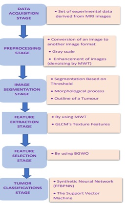 Figure1: Diagram of the proposed Classifier's Principal Block.
The data acquisition stage
The experimental data set used in this paper consists of MRI images collected from 979 MR brain images (250 normal and 729 abnormal). The database already contains 177 Glioma types, a Malignant, 551 meningioma, and a pituitary type, a Benign. These data were collected from the Kaggle website, an online community of data scientists and practitioners of machine learning. It is essential to know that in the web-based data-science environment, Kaggle enables users to locate and post data sets and explore and construct models. The acquisition will take into account the patient's MRI scan images, which can be color, Grayscale, or intensity images. Next, these images will be displayed with a standard size of 220×220 pixels. For the color image case, it will be converted into a Gray- scale image using a large matrix. The entries of this matrix are numerical values in the range of 0 to 255.
The pre-processing stage
In this Pre-processing stage, firstly, the noise will be removed. Here several types of spatial filters, linear or nonlinear, were used. Mostly here, it included median filters noise removal type. In contemporary MRI scans, the likelihood of noise is extremely low. This is where the RGB to grey conversion and reshaping are done. It may arrive due to the thermal effect. Increased accuracy and compatibility with human or machine vision systems are two primary goals of pre-major image processing [2]. The grayscale image is helpful for various tasks, including image segmentation, feature extraction, and image classification [15]. The (rgb2gray) function of the MATLAB software is used to convert RGB images to grayscale images. Sometimes, noise in MRI images should be disregarded and eliminated. This noise is caused by the high frequency of radio waves and the patient's movements during the MRI [2].
However, noise reduction should not damage the image's edges or affect its clarity and quality. Image smoothing was performed here. This is necessary in order to simplify the image under consideration while measuring the valuable information. The goal is to further reduce other types of noise, such as text noise or useless details, without producing further distortion, simplifying the forthcoming analysis.
So, for this reason, the Multi Wavelet Transform (MWT) was used. The wavelet thresholding approach for obtaining an image from noisy data was born out of breakthroughs in wavelet theory. Multiwavelets, also known as scalar wavelets, are wavelets with multiple scaling functions that enable simultaneous orthogonality, symmetry, and short support, which is not feasible with conventional wavelets. Because of this characteristic, many image processing tasks, including denoising, are better suited to multiwavelets [11]. Pre-filtering on the input image is performed to convert scalar coefficients into vector coefficients for Multiwavelet decomposition, shown in Figure 2. The standard Multiwavelets-based functions used here for decomposition are of the pre- filtered Geronimo-Hardin-Massopust (GHM) type. Infarct, there are two types of multiwavelets:
- Orthogonal types such as Geronimo-Hardin-Massopust (GHM)
- Bi-Orthogonal types such as Bi-Orthogonal Hermite [11]
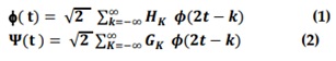 Ψ (t) is a Multiwavelet, and f (t) is a multiscaling function. Note, that (H ) and (GK ) is matrix filters, i.e, HK and GK are r× r matrices for each integer k. Because of the matrix elements, these filters have more freedom than a normal scalar wavelet filter. Extradegrees of freedom in multiwavelet filters can be utilized to include key features such as orthogonality, symmetry, and high-order approximation in the filters. What we're trying to do is figure out how to best utilize these additional degrees of freedom." Multifilter construction approaches are already being developed to make use of them [12-14]. The objective of this multiplicity is to achieve the characteristics described below [1].
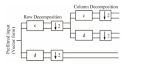 Figure 2: A filter bank including a low pass filter.
The GHM filter suggested by Geronimo, Hadrian, and Massopust is a well-known multiwavelet filter. The GHM basis offers a combination of orthogonality, symmetry, and compact support that is unmatched by any other scalar wavelet basis [15]. When the GHM, a particular kind of MWT, processes the indicated image, it divides it into multiple levels of image or parts (16 parts), and we then take the position (L1L1), which denotes that the image is significantly clearer than the input image and will be clear package sequences when using the tumor detection method(see Figure 3 to Figure 5).
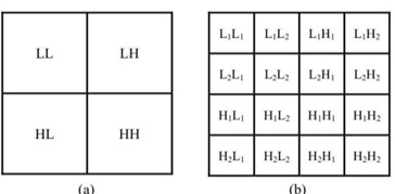 Figure 3: The image sub-bands after first level of Multiwavelet decomposition.
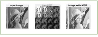 Figure 4: After applying GHM to the image.
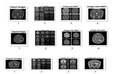 Figure 5: Brain MRI after MWT.
The image segmentation stage
The segmentation stage is essential for analyzing image characteristics because it influences the accuracy of the classification process. There are several types of skins and textures; hence it is challenging to select a proper segmentation. As well as there are several types of lesion shapes, sizes, and colors, furthermore, In certain circumstances, the skin and the lesion merge seamlessly , and some lesions have irregular boundaries. To solve this problem, different algorithms were proposed. Among them are supervised and unsupervised, thresholding, region-based or edge-based classification techniques. They aim to remove unwanted parts, consisting of several operations, namely, Dilatation and erosion, opening and closing of images.
The conclusion has been made as to whether this MRI image contains a tumor and if it is normal or abnormal. Image segmentation is a technique for separating the significant component of the brain from unwanted bits. To remove these parts, thresholding and a structural element are applied. Thresholding takes the image (converted to grayscale) as input and yields a binary image as output. Each pixel in the image must have a threshold computed. The foreground value is used if the pixel value is less than the threshold; otherwise, the background value is used [15] . To implement thresholding in Matlab: image to BW image by threshold = 0.5.
Using the BW label command each disconnected component will be labeled by a unique number. Figure 6 shows the application of these steps on a given image.
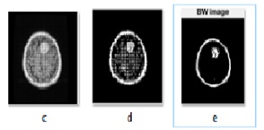 Figure 6: Segmented Image.
Morphological operations
Morphology is the study of shapes and the creation of border regions from images of brain tumors. Morphological operation is the process of rearranging the order of pixel values. It functions by arranging pieces and uploading photographs. Structure elements are qualities that look at a particular feature of interest. The processes used here are the principles of dilation and erosion. Dilation Erosion eliminates pixels from the boundary region, whereas the process adds them. As well, Pixels from the object's boundary region will be removed. As a result, the plan elements were in charge of these operations. Dilation evaluates each value and selects the best one. Erosion represents pixel values near the input image. Erosion, on the other hand, selects the lowest value by comparing each pixel value in the input image [16]. To implement Morphological using a structural, morphological element requires the following:
- Selection of strel object, a flat morphological, structural element needed for morphological dilatation and
- Achievement of the operations of Morphological Dilation and
Note that dilatation and erosion are the two most fundamental morphological processes. While dilation adds pixels to an image's object boundaries, erosion subtracts them from them. The number of pixels added or subtracted from an image's objects depends on the size and shape of the structuring element employed to analyze the image [17].
The feature extraction
Texture analysis successfully distinguishes natural from irregular tissues for human perception and machine learning. It provides a difference between invisible normal and malignant tissues. It improves the effectiveness of early diagnosis by selecting effective quantitative features. The statistical textural analysis is used to extract information from image intensities that have been segmented. In the subsequent step, textural characteristics were derived from the MWT decomposition's LL sub bands' GLCM components.
By reducing the data representation pattern, extracting features entails the extraction and transformation of input data details into many features, also known as a feature vector. To fulfill the classification task, the components set will extract the input data (image) retrieval [2]. The most used algorithms for extracting features from MRI brain images are the Discrete Wavelet Transform (DWT), the Gabor filter, and the Gray Level Co-occurrence Matrix (GLCM) [18]. This paper used a hybrid method (MWT+GLCM). DWT provides local signal time-frequency information with cascaded high-pass and low- pass filter banks to hierarchically retrieved features, enabling the extraction of the most relevant features of varied pathways and dimensions [19]. The concept of Multiwavelet was born out of the generalization of scalar wavelets [1,2]. Multiple wavelets and scalar functions are used instead of a single scalar one. Creating Multiwavelets is now far more customizable because of this feature. Because of this, unlike scalar wavelets, Multiwavelets can collect properties such as orthogonality, symmetry, higher order of vanishing moments, and compact support all at once. The Gray Level Co-occurrence Matrix (GLCM) has been demonstrated to be superior in terms of the dimension of the feature vectors. It is hence more suitable for MRI image categorization. The GLCM methodology is a statistical method for extracting texture information from the image [20]. It is presumed that the texture of normal tissues and that of malignant tissues are vastly different. These features are contrast, correlation, energy, and homogeneity retrieved from the GLCM matrix [18]. Classification is improved by selecting a suitable set of characteristics. The following matrices' properties were also gleaned: mean, standard deviation, entropy, RMS, variance, kurtosis, and skew.
The feature selection
Feature selection gives a method for detecting the essential traits and deleting the unnecessary (redundant) ones. Reducing data dimensionality, enhancing prediction performance, and gaining a thorough grasp of the data are the objectives of feature selection. In real-world applications, data representation frequently employs an excessive number of redundant features, meaning that specific characteristics can fill the role of others, and extra features can be eliminated. Moreover, the relevant (interdependence) characteristics influence the output and contain crucial information that will be obscured if any of them are omitted [21].
Previously, in a high-dimensional space, a thorough search for the best traits (features) may have proved unfeasible. Numerous studies attempt to treat feature selection as a combinatorial optimization issue, in which the set of characteristics that leads to the best feature space separability [20] is the optimal set of features. The objective function can be the classification accuracy or any criterion that considers the optimal compromise between attribute extraction computational burden and efficiency [22]. The goal of feature selection in data mining, machine learning, and pattern recognition is to reduce the dimensionality of feature space, improve the anticipated accuracy of a classification method, and improve the visualization and comprehension of the induced concepts [23]. In this paper, Gray Wolf Optimization is used for selecting features. Mirjalili and his colleagues created the Grey Wolf Optimizer (GWO) in 2014, a new metaheuristics optimization method [24]. Typically, grey wolves live in packs of five to twelve individuals. GWO imitates the hunting and searching for prey behavior of grey wolves in the wild. The population of GWO is divided into alpha, beta, delta, and omega. The alpha wolf is the chief decision-maker in the pack. The beta wolf is the second leader of the pack, grouping the alpha in decision-making and other tasks. The delta wolf is the third pack leader, ruling over the omega wolves. The names of the three ideal GWO solutions in terms of mathematics are alpha ( ), beta (ß), and delta ( ), in that order. The remaining quantity is assumed to be omega. In GWO and charge of the hunting procedure while following these three leaders [25].
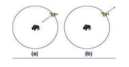
Gray Wolves encircling the prey, where the encircling behavior is model as:
 Where t = current iteration.
X(p)= position of the prey.
X= position of the gray wolf.
A.C vectors can be calculated as:
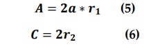 r1,r2 random vectors rang {0,1}.
Component a: Linearly decreased from 2 to 0 throughout the iteration (figure 7 to figure 8).
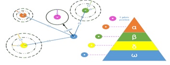 Figure 7: The Main Steps of Gray Wolf Hunting.
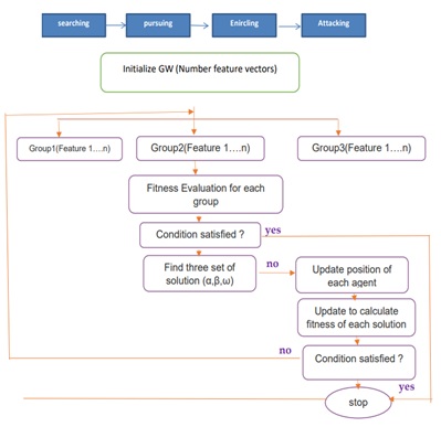 Figure 8: GWO algorithm.
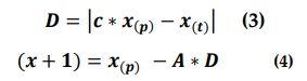
The above equations (3 & 4) are used to update the gray wolf position of the prey. Different places around the best search agent can reach. r1, r2 allows the wolf to reach any position between 2 particular points.
- -1>A > 1 means X near the prey and inside its
- A < 1 OR A > -1 which means X is far from the pray and outside of the prey
Update the position of the gray wolves as
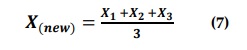 Where X1 , X2 and X3 are calculated as follows:
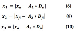 where xα?, xβ and represent the positions of alpha, beta, and delta at iteration t: A1, A2 and A3 are computed according to Equation (5): and Dα , Dβ and Dδ are specified according to Equations (11),(13) respectively.
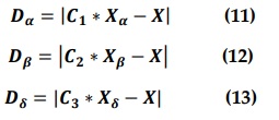 Where C1 C2 and C3 are computed according to Equation (6).
GWO is mostly intended to solve continuous optimization problems. A binary version of GWO is necessary for binary optimization issues, including feature selection [19]. Have recently presented two unique binary grey wolf optimizations (BGWO1 and BGWO2) to address feature selection difficulties. The functionality of BGWO1 and BGWO2 is discussed below [25].
Model 1 Of The Binary Grey Wolf Optimization (BGWO1)
BGWO1 uses the crossover operator to update the position of the wolf as follows for the first approach:
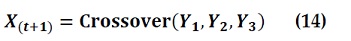 where Crossover (Y1, Y2 and Y3) is the solution crossover operation and Y1, Y2 and Y3 are the relevant binary vectors affected by the move of alpha, beta, and delta wolves. Equations (26), (29), and (32) are used in BGWO1 to define Y1, Y2 and Y3
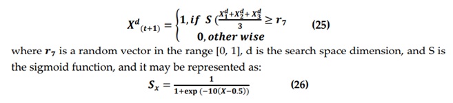
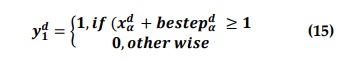 in where xα d is alpha's position, d is the dimension of the search space, and bestepα d exemplifies the binary step that can be stated as;
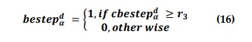 Where r3 is a random vector in the range [0, 1], and cbestepα d is the continuous-valued step size that may be determined as shown in Equation (17).
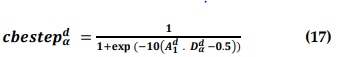 Where A1 d and Dα d are calculated using Equations (5) and (11). Following the acquisition of Y1, Y2 and Y3, the wolf's new position is updated using the crossover operation, as follows
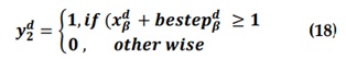

 Where d is the dimension of the search space and r6 is a uniformly distributed random number between 0 and 1[25].
Model 2 For Binary Grey Wolf Optimization (BGWO2)
In the second method, BGWO2 updates the wolf's position by transforming the position into a binary vector, as illustrated in Equation (19).
 In comparison to other metaheuristics optimizations, BGWO has the advantage of being simple, versatile, and adaptive [25] (Table 1 and Table 2).
|
feature |
image 1 |
image 2 |
image 3 |
image 4 |
image 5 |
|
contrast |
0.640441176 |
0.841636029 |
0.856311275 |
1.009375 |
0.994454657 |
|
correlation |
0.910233527 |
0.860784547 |
0.868071328 |
0.869570846 |
0.804866517 |
|
energy |
0.528243432 |
0.386076165 |
0.357839957 |
0.278508595 |
0.163992011 |
|
homogenity |
0.862152194 |
0.817836572 |
0.807137532 |
0.758822618 |
0.738226431 |
|
mean |
0.162361274 |
0.175856667 |
0.188811349 |
0.234618266 |
0.234421533 |
|
standare.dev |
0.266775535 |
0.245783908 |
0.257310639 |
0.281463718 |
0.209619171 |
|
entropy |
5.251225266 |
5.701856848 |
5.733029333 |
5.856789176 |
7.025618817 |
|
RMS |
0.234854887 |
0.242653785 |
0.258833326 |
0.309300231 |
0.283078792 |
|
variance |
0.051088124 |
0.042541337 |
0.046497383 |
0.053983453 |
0.03106896 |
|
smoothness |
0.999906028 |
0.999913239 |
0.999919192 |
0.999934968 |
0.999934913 |
|
kurtosis |
6.511363615 |
5.663715362 |
6.204270751 |
4.373772738 |
4.858106247 |
|
skewness |
1.943795806 |
1.612713698 |
1.679877484 |
1.210404933 |
1.205599953 |
|
idm |
188.8586861 |
155.7107606 |
210.9574286 |
212.22568 |
221.7859271 |
Table 1: Feature extracted by (MWT+GLCM) to 5 images.
|
feature |
image 1 |
image 2 |
image 3 |
image 4 |
image 5 |
|
energy |
0.528243432 |
0.386076165 |
0.357839957 |
0.278508595 |
0.163992011 |
|
homogenity |
0.862152194 |
0.817836572 |
0.807137532 |
0.758822618 |
0.738226431 |
|
mean |
0.162361274 |
0.175856667 |
0.188811349 |
0.234618266 |
0.234421533 |
|
entropy |
5.251225266 |
5.701856848 |
5.733029333 |
5.856789176 |
7.025618817 |
|
RMS |
0.234854887 |
0.242653785 |
0.258833326 |
0.309300231 |
0.283078792 |
|
kurtosis |
6.511363615 |
5.663715362 |
6.204270751 |
4.373772738 |
4.858106247 |
|
skewness |
1.943795806 |
1.612713698 |
1.679877484 |
1.210404933 |
1.205599953 |
Table 2: Feature Selection by (BGWO) to 5 images.
Stage Of Tumor Classification
Classification is the categorization of a given input by an appropriate classifier. The purpose of classification is to label each MR brain image based on certain visual characteristics. The structure, architecture, and design of a classification system require the selection and calculation of features extracted from the images to be classified as indicated in Figure 9.
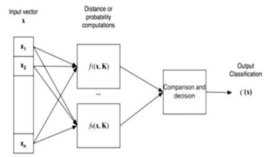 Figure 9: Structure of the Image Classification System.
Support Vector Machines
SVM was used to identify the input image as Benign or Malignant. SVM is a method for solving two-class problems that is systematic. The SVM classifier is widely used in research because it performs well in pattern recognition and image processing applications [15].
Support Vector Machines (SVMs) is a potent supervised learning technique that may be utilized in classification and regression studies for pattern recognition, data mining, and other applications, and machine learning. Cortes and Vapnik invented SVM in 1995. Numerous studies on SVM have been undertaken, such as a flexible support vector machine for regression and an evaluation of fly rock phenomena based on blasting operation using SVM [26]. SVM classifications are classified into two types: linear and non-linear [27]. The kernel function, which directly calculates the dot product in the feature space, is used to allocate the input vectors to the feature vector. The hyperplane is formed in a two-dimensional space by maximizing the distance between the two classes and completing the training sets. This hyper plane is utilized to classify vectors of unknown (testing) items [2].
Artificial Neural Network
One of the primary objectives of Artificial Neural Networks is the processing of information comparable to humor interaction. In reality, neural networks are used when brain capabilities and idealistic machines are required. The benefits of neural network information processing stem from its capacity to identify and model nonlinear data interactions [27]. An ANN consists of a number of fundamental groups known as "neurons" or artificial neurons that are interconnected and process information in simultaneously, likewise called parallel distributed processing systems or linking systems [2]. The feed-forward back propagation network (FFBPN) employed in this study, which is one type of artificial neural network due to its ease of use, has a large number of learning algorithms that may be applied to the training of the multilayer neural network.
Configure the neural network as follows
Launch (nn tool) package through MATLAB command. Import the input layer, which is comprised of 13 neurons dependent on categorical variables and numerical features derived using a gray-level co-occurrence matrix (GLCM) to represent data input. (originating from the workspace) One neuron represents the target data vector in the import output layer. (originating from the workspace) Determine one hidden layer consisting of three neurons through trial and error Configure the primary Training parameters utilized by the network for FFBPN. Configure activation function tensioning (sigmoid) Minimum threshold for gradient of 0.1 10-10 Maximum number of 1000 epochs.
Target for sum-squared error of 0.001 Distribution constant 1 Time limit for training infinity. maximum of 10 failed validation checks. Run to the train system.
Results
Figure 10 shows the results of the experiments done with the work method exhibited for the segmentation result and extracted tumor region. In Figure 9, the training network for the FFBPN was shown. Fig 10 shows the performance of the network (Table 3).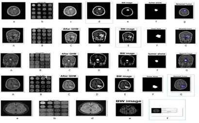 Figure 10: Performance of the network
|
Authors |
Features |
Classification Algorithm |
Accuracy |
|
2017 [6] |
Extracted 4 textural features by GLCM method |
SVM-based classification |
95% |
|
2018[7] |
Extracted 5 textural features by GLCM and DWT |
PNN classifier |
Nearly 100% was achieved for trained and95% for tested |
|
2019 [8] |
9 features by the GLCM method |
SVM, FFNN, and ELM |
92.99%,89.41% and 90.20% |
|
2020 [9] |
Extracted 5 textural features by GLCM |
SVM |
90% |
|
2020[2] |
Extracted 13 textural features by GLCM method |
SVM and FFBPN |
93% and 97% |
|
Propose Algorithm |
Extracted 13 textural features by GLCM method and MWT then selected 6 features by BGWO |
SVM and FFBPN |
100% and 100% |
Table 3: Com parison of results with prior efforts on brain tumor detection and categorization.
For the training dataset, the FFBPN was 100% accurate, for the testing dataset it was 100% accurate and for the validation dataset it was 100% accurate. So, everyone agrees that the overall method is 100 percent accurate. Only for 25 epochs has the given accuracy been seen (Figure(11-13)).
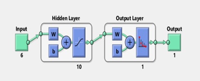 Figure 11: Training dataset.
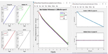 Figure 12: SVM classifier.
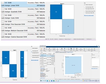 Figure 13: SVM and Artificial Neural Networks.
Conclusion
MWT, BGWO, SVM and Artificial Neural Networks were used to develop an automated approach for MRI brain tumor detection. In two phases, MWT is employed (in pre-processing & feature extraction). Analysis of statistical features was utilized to extract features from images; attributes determined using Graycomatrix features based on the (GLCM) of the images. BGWO was used to select optimal features. The feed-forward backpropagation network with supervised learning has been used to classify images as benign, or malignant in artificial neural networks. And the appropriate features were employed as input variables for the FFBPN before training the network and evaluating its performance. The suggested method, FFBPN, achieves the best results by detecting and classifying brain cancers based on the extraction feature with 100 percent accuracy, so the SVM has a high accuracy 100%. The suggested approach classifies the MRI images of brain tumors efficiently.
References
- Zhang Y, Wu L (2012) An MR brain images classifier via principal component analysis and kernel support vector Prog Electromagn Res 130: 369-388.
- Abd Alreda B, Khalif H, Saeid T (2020) Automated Brain Tumor Detection Based on Feature Extraction from the MRI Brain Image Analysis. Iraqi J Electr. Electron Eng 16: 1-10.
- Transform M, Function A, Network W (2011) Multiwavelet Transform And Multi-Dimension-Two Activation Function Wavelet Network Using For Person 11: 46-61
- Subramanian B, Ramasamy A, Rangasamy K (2014) Performance comparison of wavelet and multiwavelet denoising methods for an electrocardiogram signal J Appl Math
- Abraham A, Krömer P, Snášel V (2015) Afro-European Conference for Industrial Advancement: Proceedings of the First International Afro-European Conference for Industrial Advancement AECIA 2014. Adv Intell Syst Comput 334: 1-13.
- Miranda E, Aryuni M, Irwansyah.E (2016) A survey of medical image classification Int Conf Inf Manag Technol ICIM Tech 56-61.
- Bahadure NB, Ray AK, Thethi HB (2017) Image Analysis for MRI Based Brain Tumor Detection and Feature Extraction Using Biologically Inspired BWT and SVM. Int J Biomed Imaging
- Varuna Shree N, Kumar TNR (2018) Identification and classification of brain tumor MRI images with feature extraction using DWT and probabilistic neural Brain Informatics 5: 23-30.
- Kumar P,Vijay Kumar B (2019) Brain tumor MRI segmentation and classification using ensemble classifier. Int J Recent Technol Eng 8: 244-252.
- Umary A, Kaur H (2020) Automatic Brain Tumour Diagnosis and Segmentation: Based on SVM Algorithm. Int J Innov Technol Explor Eng 9: 1079-1084.
- Al Jumah A, Gulam Ahamad M, Amjad Ali S (2013) Denoising of Medical Images Using Multiwavelet Transforms and Various Thresholding Techniques. J Signal Inf Process 4: 24-32.
- Mahmoud WA, Loay A, Rasheed M (2010) 3D Image Denoising by Using 3D Multiwavelet. Scientific research 7: 108-136.
- Al-Helali HA, Mahmmoud AH, Ali (2012) A Fast Personal Palmprint Authentication Based on 3D-Multi-wavelet Transformation.Trans. J Sci Technol 8: 1-10
- Waleed P, Mahmoud A (2011) A Smart Single Matrix Realization of Fast Walidlet Transform 1.
- Alfonse M, Salem M (2016) An Automatic Classification of Brain Tumors through MRI Using Support Vector Machine Egypt. Comput Sci J 3: 1110-2586.
- Xu L, Gao Q, Yousefi N (2020) Brain tumor diagnosis based on discrete wavelet transform, gray-level co-occurrence matrix and optimal deep belief network Simulation 11: 867-879.
- Al-jawher WA, Awad SH (2022) Materials Today: Proceedings A proposed brain tumor detection algorithm using Multi wavelet Transform (MWT) Mater. Today Proc 13: 102-112
- Hamiane M, Saeed F (2017) SVM classification of MRI brain images for computer- assisted diagnosis. Int J Electr Comput Eng 5: 2555-2564.
- Icke G, Kamarthi SV (2005) Feature extraction through discrete wavelet transforms coefficients. Intell Syst Des Manuf 6: 599903.
- Zulpe N, Pawar V (2012) GLCM textural features for Brain Tumor Classification. Int J Comput 3: 354-359.
- Emary E, Zawbaa MH, Hassanien AE (2016) Binary grey wolf optimization approaches for feature selection. Neurocomputing 172: 371-381.
- Nakamura R, Pereira L, Costa K, Rodrigues D, Papa J (2012) BBA: A binary bat algorithm for feature selection Brazilian Symp Comput Graph. Image Process 291-297.
- Ibraheem al-jadir WA (2020) A Grey Wolf Optimizer Feature Selection method and its Effect on the Performance of Document Classification Problem. J Port Sci Res 4: 2.
- Lippert AM, Reitz RD (1997) Modeling of multicomponent fuels using continuous distributions with application to droplet evaporation and sprays. SAE Tech 69: 46-61.
- Too J, Abdullah AR, Saad NM, Ali NM, Tee W (2018) A new competitive binary grey wolf optimizer to solve the feature selection problem in EMG signals classification Computers 7: 4.
- Uzer MS,Yilmaz N, Inan O (2013) Feature selection method based on artificial bee colony algorithm and support vector machines for medical datasets classification Sci World J
- Hussein EM, Mahmoud D, Mahmoud A (2012) Brain Tumor Detection Using Artificial Neural Networks J Sci Technol 13: 31-39.
Citation: Mahmoud Al-Jawher A, Awad Al-taee SH (2022) Precise Classification of Brain Magnetic Resonance Imaging (MRIs) using Gray Wolf Optimization (GWO) J Brain Neursci 6: 021
Copyright: © 2022 Waleed A Mahmoud Al-Jawher, et al. This is an open-access article distributed under the terms of the Creative Commons Attribution License, which permits unrestricted use, distribution, and reproduction in any medium, provided the original author and source are credited.