Prevalence and Determinants of Stunting and Wasting On Children Under-Five Years in Ethiopia

EDHS: Ethiopian Demographic and Health Survey

In developing countries, child stunting and wasting is the leading public health problem and is a major cause of child morbidity and mortality. For stunting and wasting, under-five children are the most vulnerable. The nutrition of infants and young children is a major concern to any society [1]. According to World Health Organization (WHO), child stunting and wasting is considered by height for age and weight for height indexed respectively [2]. 

In sub Saharan Africa the prevalence of stunting is declining but is still over 30% [3]. Several African countries have updated their national nutrition policies, strategies and action plans [4] in order to address malnutrition. Ethiopia has known shows potential progress in dropping levels of malnutrition over two past decades. However, the baseline levels of malnutrition remain so high that the country still needs to continue substantial investment in nutrition. According to Ethiopian Demographic and Health Survey (EDHS), there is a substantial variation of under-five children nutrition in Ethiopia [5-6]. 

At the policy and program level, Ethiopia has many strategies and programs to reduce levels of stunting and wasting as part of its national development agenda. The Government of Ethiopia through the Ministry of Health also launched the health extension program in 2003 to achieve the country’s progress in meeting the Millennium Development Goals (MDGs). The health extension workers are mainly to improve access to care in rural communities. They spend 15% of their time with infants and children under age 5 [7]. All of these listed efforts have brought positive impact in improving food and nutrition security [8]. 

In Ethiopia, child malnutrition is one of the most serious public health problems and the highest in the world [9] and has a significant impact on communities, in particular for women and children. Millions of children die of severe acute malnutrition each year and poor nutrition prevents many children and adults from ever reaching their full mental and physical capacity. Among the factors that cause child malnutrition in Ethiopia are insufficient availability of food, inadequate provision of a healthy environment, such as sanitation and hygiene, women’s status concerning decision-making power, and factors related to political economy [10].  By the taking the problem into the consideration, child stunting and wasting problem is faced by complex interaction of a multitude of factors. Especially, social factors such as educational influence. That means, children born from uneducated women not suffer from stunting and wasting problems. The determinants of stunting and wasting include the place of residency, the number of under-five children in households, birth order, sources of improved drinking water, and toilet facility [11]. Most studies also found that sex of a child, child age, and household wealth index were found to be significant factors on under-five children stunting, wasting, and underweight [12]. Therefore, the main objectives of this study were to assess the prevalence and the determinants of stunting and wasting on children under-five in Ethiopia using the Ethiopian Mini Demographic and Health Survey [13].

Data Source                                                                       

The study used cross-sectional secondary data which is obtained from the Ethiopian Mini Demographic and Health Survey [13]. The survey was conducted from March 21, 2019, to June 28, 2019 [13].  

Study population 

Thus, the study populations for this study were all children under-five in Ethiopia. From total of 5,753 under five children, the researchers used 3880 under five children with complete anthropometric measurements for the final analysis by making the rearrangements in terms of height-for-age and weight for height of the children’s [13]. 

Study variables 

As demonstrated in the literature review, socio-economic, demographic, health and environmental characteristics are considered as the most important determinants of stunting and wasting among under-five children in Ethiopia. 

Outcome variable 

For this study, the outcome variable was the two anthropometric indicators mostly used for monitoring malnutrition in children under-five: stunting (height for-age) and wasting (weight-for height) [14].

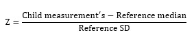Where,

Child’s measurement = height or weight of a given child at age X

Reference median = mean or 50th percentile of the reference population at age X

Reference SD = standard deviation of the reference population at age X

Independent variables

To analyze the child stunting and wasting among under-five, the study considers the following characteristics as independent variables 

Methods of data analysis 

In this study both exploratory (descriptive) and inferential statistical data analysis methods were employed. 

Exploratory data analysis 

Descriptive statistics were used to observe a possible link between explanatory variables and child nutritional outcome variables. Univariate associations between potential covariates and the response variable were assessed using frequency tables and by fitting each predictor with each response univariately. Descriptive statistics was used like frequency table, percent between explanatory variables with stunting and wasting. 

Statistical models and Methods 

Multivariate Data analysis 

Multivariate analysis is a set of techniques used for analysis of data sets that contain more than one variable, and the techniques are especially valuable when working with correlated variables is used to study more complex sets of data than what univariate analysis methods can handle [15]. Most multivariate analysis involves a dependent variable and multiple independent variables [16]. Multivariate response was recommended when there is a correlation between two response variables differs from zero [17]. 

Component of multivariate data analysis 

Principal component analysis 

Reducing the number of variables of a data set naturally comes at the expense of accuracy, but the trick in dimensionality reduction is to trade a little accuracy for simplicity. Because smaller data sets are easier to explore and visualize and make analyzing data much easier and faster for machine learning algorithms without extraneous variables to process. So to sum up, the idea of PCA is simple and reduce the number of variables of a data set, while preserving as much information as possible [18]. 

Mathematical expression of principal component analysis

Such that

Y_k’s are uncorrelated (orthogonal)

Y₁ explains as much as possible of original variance in dataset

Y₂ explains as much as possible of remaining variance

Proportions of total population variance

Factor analysis

Factor analysis has been used in two data analytic contexts: in a confirmatory manner designed to confirm or negate the hypothesized structure, or to try to discover a structure, in which case the analysis is called exploratory. The results of factor analysis (with factor loadings greater than 0.4 in an absolute) are presented. The Principal Component Factor Analysis was done considering the socioeconomic, demographic, health and environmental variables. The component loadings represent the correlation between the components and original variables. In this study, we concentrate on loadings above 0.4 or below -0.4 (sometimes 0.5 as a cutoff) and components/factors are named based on the highest loadings [19]. Factor Analysis is closely related to Principal Component Analysis, and often confused with it. Rather than a mapping into lower dimensions, or, equivalently, a rotation, that is PCA, FA aims to fit an explicit model.

Where X is the data matrix with covariance matrix Σ, ε is the ‘error’ containing, in FA jargon, the unique factors, f are the common factors, and Γ contains the factor loadings. Also, it is assumed that f and ε have mean zero and are uncorrelated. 

Unlike the case with PCA, the scores of the first, say, two factors are different when fitting an FA model with two or three factors, a possible difficulty in the interpretation. Unfortunately, there is no analytical way to arrive at the factorial analysis solution, so that a number of different algorithms are in use today. The most important ones are the maximum-likelihood approach and principal factor analysis.

Determining the number of factors

Priori determination 

Sometimes, because of prior knowledge, the researcher knows how many factors to expect and thus can specify the number of factors to be extracted beforehand [20]. 

Determination based on eigenvalues 

In this approach, only factors with Eigen values greater than 1.0 are retained. An Eigen value represents the amount of variance associated with the factor. Hence, only factors with a variance greater than 1.0 are included. Factors with variance less than 1.0 are no better than a single variable, since, due to standardization, each variable has a variance of 1.0. If the number of variables is less than 20, this approach will result in a conservative number of factors [20]. 

Determination based on scree plot. 

A scree plot is a plot of the Eigenvalues against the number of factors in order of extraction.

Experimental evidence indicates that the point at which the scree begins denotes the true number of factors. Generally, the number of factors determined by a scree plot will be one or a few more than that determined by the Eigenvalue criterion [20].

Goodness of fit test of multivariate model 

Manova tests 

The following are the principal test statistic for the multivariate analysis of variance Wilk’s determinant ratio;

Canonical correlation analysis

Computationally a canonical correlation analysis was performed to exploring the relationships between multivariate sets of variables (vectors), all measured on the same individual and that determined the successive functions and canonical roots. Classification was then possible from the canonical functions. Individuals were classified in the groups in which they had the highest classification scores [21]. This analysis further provided a percentage of overall correct classification.

Exploratory factor analysis

Factor analysis could be described as orderly simplification of interrelated measures. Traditionally factor analysis has been used to explore the possible underlying structure of a set of interrelated variables without imposing any preconceived structure on the outcome [19]. By performing exploratory factor analysis (EFA), the number of constructs and the underlying factor structure are identified.

Multivariate model building process

The primary part (stages one to stages three) deals with the analysis objectives, analysis style concerns, and testing for assumptions. The second half deals with the problems referring to model estimation, interpretation and model validation.

Parametric estimation of multivariate multiple linear regression model

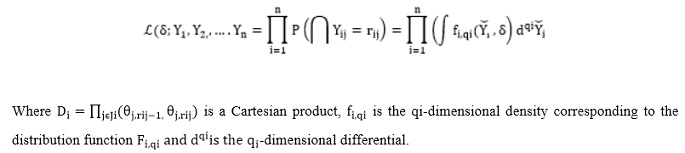
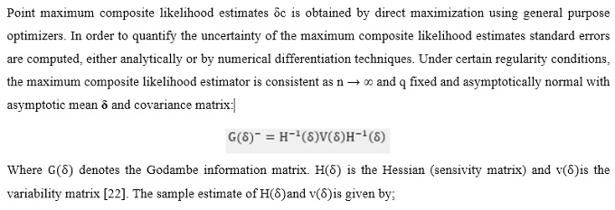
In order to estimate the model parameters we use a composite likelihood approach, where the full likelihood is approximated by a pseudo-likelihood which will be constructed from lower dimensional marginal distributions, more specifically by “aggregating” the likelihoods corresponding to pairs and triplets of observations, respectively. In the presence of ignorable missing observations, the composite likelihood will be constructed from the available outcomes for each subject i. In contrast to [22-23] for the pairwise approach we include univariate probabilities if only one outcome is observed. Similarly, for the tripletwise approach univariate and bivariate probabilities are included if q_i is less than three. 

For the sake of notation we introduce an n ×q binary index matrix Z, where each element z_ij takes a value of 1 if j ∈ J_i and 0 otherwise. The pairwise log-likelihood is given by:

If, for the case of no missing observations, the errors follow a q-dimensional multivariate normal or multivariate logistic distribution, the lower dimensional marginal distributions F_i, _qi are also normally or logistically distributed.

In the sequel we denote by fi,₁, fi,₂ and fi,₃ the uni-, bi- and trivariate densities corresponding to F_i,₁, F_i,₂ and F_i,₃. Hence, the marginal probabilities can be expressed as:

For all correlation matrices we use the spherical parameterization and transform the constrained parameter space into an unconstrained one. The spherical parameterization for covariance matrices has the advantage over other parameterizations in that it can easily be modified to apply to a correlation matrix.

Descriptive statistics 

The main purposes of the present descriptive analysis were to describe the analysis among the categorical explanatory variables on under-five children in Ethiopia through the percentage values. The data were entered into SPSS windows version 20 for the analysis. 

Of the total 3880 under-five children included in the study, of them, 1953 (50.3%) were males whereas 1927 (49.7%) females. From the child residency 3191 (82.2%) were children live in rural whereas 689(17.8%) were children live in urban area. From the child mother 2457 (63.3%) were illiterate, 967 (24.9%) were primary levels, 294 (7.6%) were Secondary level and 162(4.2%) were higher education level. With regard to the marital status of the sample respondents, 7 (0.2%) respondents were never in union, 3755 (96.5%) respondent were Married/living with partner, and 118 (3.0%) respondents were separated. When we consider the variable wealth index, the poorest were 1400 (36.1%), poorer were 650 (16.8%), middle were 531 (13.7%), Richer were 520 (13.4%) and richest 779 (20.1%) (See Table 1).

Table 1: Results of Descriptive statistics and bivariate analysis.

Inferential Statistical Analysis 

Correlation between the response variable (Stunting and wasting) 

Table 2 shows that the relationship between the response categories. This indicates that there is the correlation between two response variables (Stunting and wasting) because the correlations between the responses are differ from zero. Since there is the correlation between the response categories, then the multivariate analysis are the best fit models for this given EMDHS data. 

Table 2: The correlation between the response categories under-five.

Multivariate component data analysis

Factorial analysis 

From Table 3 we can just we reject the null hypothesis. On the other hand, the confidence ellipsoid for β can be easily contracted with the one at a time t value t (n – k – 1) at the given significance level. Thus, the data were checked for Bartlett‘s test of Sphericity to see that the correlation matrix is an identity matrix; the test shows that the factor model is appropriate since (p-value < 0.0001). Therefore, the hypothesis of our correlation matrix is an identity matrix, which would indicate that our variables are unrelated and therefore unsuitable for structure detection. These Small values of the significance level indicate that a factor analysis may be useful with our data.

Table 3: KMOs and Bartlett’s Tests for Factor Analyses.

For principal components extraction, this initial eigenvalues are equal to 1.0 for correlation analyses. Extraction communalities are estimates of the variance in each variable accounted for by the components. The communalities in this table are all high or suggests the communalities above 0.4 is acceptable [24], which indicates that the extracted components represent the variables well because no any communalities are very low in a principal components extraction, thus the author may not need to extract another component (Tables 4 & 5) 

Table 4: Communalities.

Principal Component Analysis

Table 5: Total Variance Explained.

Depending on the correlation matrix and communalities, of all 3880 observed items, using principal component extraction and Varimax rotation, the study found that eight underlying common factors for factor analysis that constituted or explained 59.646% of the total variability in the corresponding original observed variables with only a 40.354% loss of information. This suggests that eight latent influences are associated with service usage, but there remains room for a lot of unexplained variation (Table 6).

Table 6: Factor loadings (pattern matrix) and unique variances.

In the above table, the values that we consider large are in boldface. The following statements are based on this criterion: 

Factor 1 is correlated with Region (and Mother's educational level, Type of place of residence, Wealth index of mothers, Fathers education level, and Birth order number. The author can say that the first factor is primarily a measure of these variables. 

Factor 2 is correlated with Duration of breastfeeding and Child's age (in months). The author can say that the second factor is primarily a measure of these variables.

Factor 3 is correlated with Sex of household head and Current marital status. The author can say that the third factor is primarily a measure of these variables. 

Factor 4 is correlated with Preceding birth interval (in months) and Number of under-five children in the household. The author can say that the fourth factor is primarily a measure of these variables. 

Factor 5 is correlated with birth order number and Size of child at birth. The author can say that the fifth factor is primarily a measure of these variables. 

Factor 6 is correlated with type of toilet facility and source of drinking water. The author can say that the sixth factor is primarily a measure of these variables. 

Similarly Factor 7 is correlated with sex of child. The author can say that the seventh factor is primarily a measure of these variables. 

Factor 8 is correlated with type of cooking fuel. The author can say that the eighth factor is primarily a measure of these variables. 

The scree plot in Figure 1 reveals that the first eight components have Eigen values above 1, explaining at least as much of the variation as the original variables or visualizes the Eigenvalues we just saw. Again, we see that the first eight components have Eigenvalues over 1. We consider these “strong factors” and after that -component nine and onwards- the Eigenvalues drop off dramatically.

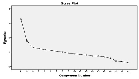 Figure 1: Scree plot of Eigen values after PCA.

Results of multivariate multiple linear regression analysis 

From the given covariates, the variables such as type of toilet facility, Sex of child, Preceding birth interval (in months), Region, Type of place of residence, Mother's educational level, Wealth index of mothers, fathers education level, mothers occupational status, Birth order number, Duration of breastfeeding, Child's age (in months), and Number of under-five children in the household are simultaneously significantly associated with stunting (Height/Age) and wasting (Weight/Height) (Table 7).

Table 7: Parameter estimates of multivariate multiple liner regression. 

A one unit change in mother’s educational level is associated with a -7.339, 1.103 unit change in the predicted value of Height/Age (stunting) and Weight/Height (wasting), respectively. A one unit change in wealth index of mother’s is associated with a -2.059, 1.507 unit change in the predicted value of Height/Age (stunting) and Weight/Height (wasting), respectively. A one unit change in child’s age (in months) is associated with a -.724, -1.643 unit change in the predicted value of Height/Age (stunting) and Weight/Height (wasting), respectively.

Assessing multivariate multiple models goodness of ft

Table 8: Multivariate Analysis of Variance (MANOVA) for the fitted model. 

The F-value column reveals that the three models are good fit or each of the two univariate models are statistically significant because the significance value or P-value ≤ 0.001.

Canonical correlation

Table 9: Eigenvalues and Canonical Correlations. 

The first canonical correlation coefficient is 9.66% with an explained variance of the correlation 79.45% and an eigenvalue of 0.00942. The second canonical correlation coefficient is 4.93% with an explained variance of the correlation % and eigenvalue of 0.00244. This is the proportion of explained variance in the canonical variates attributed to a given canonical correlation. That means, the 9.66% variation of stunting was explained by the canonical covariates, 4.93% variation of wasting was explained by the canonical covariates. Thus indicating that our hypothesis is correct – generally the variable stunting (height for age), wasting (weight for height) are positively correlated.

Accordingly, this study has tried to look into factors associated with child stunting and wasting in the study area by incorporating as many risk factors as possible. The variables such as type of toilet facility, Sex of child, Preceding birth interval (in months), Region, Type of place of residence, Mother's educational level, Wealth index of mothers, father education level, mother occupational status, Birth order number, Duration of breastfeeding, Child's age (in months), and Number of under-five children in the household are significantly associated with stunting and wasting simultaneously. 

Mother educational level is one of the most important determinants of stunting and wasting. Educated parents are more likely to employ better child-care practices as compared to uneducated parents. The study shows that higher level of mothers’ educational attainment was positively associated with under-five children stunting and wasting. Similar findings shows that the studies in the Uganda [25], Mozambique [26], and Ghana [27], the reasons include that educated women are better informed about optimal child care practices [28], have better hygiene practices [29-30], feeding [31], and childcare during illness [31-33], have a greater ability to use the health system [34], and are more empowered to make decisions [29]. In our study, however, in about two-thirds of cases (65%), the mothers had not attended formal education. According to a study done in Bangladesh, children of mothers with secondary or higher education were at a lower risk of childhood stunting (risk ratio (RR): 0.86) and wasting (RR: 0.82) as compared to children of uneducated mothers [35]. Maternal education has been associated with the better nutritional condition during pregnancy and after birth. This has been shown to be an indirect predictor of better child’s health throughout life [36]. A study done in Pakistan concluded that illiterate mothers are more likely to have poor knowledge about the nutritional requirement of their children, which results in unhealthy feeding practices. This is one of the most common reasons of child stunting and wasting among Pakistani children [37]. 

The findings of this study showed that preceding birth interval (in months) is a significant predictor of stunting and wasting. Children having birth interval less than 24 months had higher risk of being wasting as compared with children having greater than or equal to 48 month’s birth interval. This study was in line with the study conducted in Bangladesh [38]. Similar study which was conducted in Ethiopia, Nigeria, India, and Bangladesh [39] confirms this author paper results. They argued that preceding birth interval is the other important variable which is associated with child stunting and wasting. In particular, there is an inverse relationship between the length of the preceding birth interval and the proportion of children who is malnourished. This finding is also consistent with the report of Ethiopian DHS 2011 [40] and 2016 [6]. For the newborns, the larger birth interval results into better care and more time allocation for the nutrition and wellbeing [41].

This study shoes age of child is the significant factor on child stunting and wasting. Previous studies in Ethiopia have shown similar results [42]. The reason might be that as children grow older they have greater energy needs. Especially, besides stunting reflects chronic malnutrition that can be manifested after long-term nutritional deficiency, while wasting reflects acute under nutrition. As child’s age increase, there is the probability that the child will receive childhood vaccinations, which reduce exposure to disease.  

The Birth Order number is the significant factor on the under-five children stunting and wasting in Ethiopia. This finding is supported by a similar result from previous study [43]. Overall, our results suggest that high percentage of malnutrition among low birth order children could be avoided with the improvement of birth spacing as better nutritional outcome seen among children with lower birth order and longer birth interval. Although, the finding suggest that the combination of lower birth order [2-3] and lesser birth interval (<24) that often adversely affects child’s stunting and wasting. 

The factor number of children in the household is also the major significant effect on under-five stunting and wasting in this study. Increasing number children, family size increases, child wasting and stunting increases, reason underlying is this with family increase resources become scare and less nutrition and care focused to children. These findings are consistent with studies of [44] and in contrast the studies of [45]. Additionally, On the other hand, the high number of under-five children in families was more likely to be associated with under-five stunting and wasting. Various literature studies indicated that larger under-five children in households were significantly positively associated with stunting and wasting [46] and this may be because the large household size is widely regarded as a risk factor for stunting and wasting particularly for infants and young children due to food insecurity. 

Children of lowest wealth quintile were higher frequency of child stunting and wasting rather than higher wealth quintile family children due to underlying reason of less affordability of healthcare, quality nutrition and hygiene rather than rich families. These results are similar with the studies of [47]. Households with food shortage were higher prevalence of malnutrition in children rather than children adequate access of food. Adequate nutrition promotes health and resistance against diseases, while inadequate nutrition causes to increase severity of stunting and wasting. These findings are consistent with the study of [48]. 

The factor duration of breast feeding that encompassed ever breast feeding, still breast feeding, never breast feeding had a significant impact on child stunting and wasting. This may be due to the no longer time that a mother feed breast to her child at least for six months the more the child is health and gets balanced nutrients. Breastfeeding can enable eye-to-eye contact, physical closeness and emotional bonding, essential for optimal child growth and development [49]. Early initiation of breastfeeding serves as the starting point for the continuum of care for the mother and the new born that can have long-lasting effects on health and development. The findings in this study showed that more than half of the children were initiated to the breast within one hour of birth. The results do not differ much from those of general population in Kenya 58% [50]. This is because most of the children are delivered in the same hospitals as the general population thus subjected to the same health services. In low-resource settings where infection causes a large proportion of new-born deaths, exclusive breastfeeding can substantially reduce child mortality [49]. Prison set ups have been described as a low-resource setting with high cases of morbidity due to overcrowding and other aggravating factors. Mothers, who 66 deliver while in incarceration, need support to initiate breastfeeding within the first hour of birth. As a global public health recommendation, infants should be exclusively breastfed for the first six months of life to achieve optimal growth, development and health [51]. Based on a 24 hour recall most of the infants less than 6 months of age in this study had been exclusively breastfed. The current study indicated that the place of residence was associated with significant effects under-five stunting and wasting. This finding evens the finding(s) in earlier (previous) studies [51-52].  

In this study, the multivariate analysis on stunting and wasting of under-five was considered and there is a dependency between two nutritional responses. The researcher assesses the association between the two nutritional responses and suggests that it is better to take the correlation between the two responses to understand the effects of covariates on those nutritional outcomes simultaneously. The finding is consistent with the findings of the previous studies conducted in Nigeria by [53]. The Multivariate analysis was employed to determine the effects of covariates on stunting and wasting. Based on this model, the significant dependencies between stunting and wasting were noticed given other children and household characteristics. Hence, a better understanding of the association between anthropometric indicators will help in developing focused interventions to improve child health and survival. The previous study also conducted in Ethiopia and India [54-55] reported the significant association between stunting and wasting.

This study shows that the prevalence of stunting and wasting is not decreasing as well as type of toilet facility, birth interval, and duration of breast feeding are preventable factors  of stunting and wasting among under five years children in Ethiopia  Good implementation of essential nutrition action that are exclusive breast feeding, complementary feeding , improve women’s nutrition by increasing birth interval of 2 years  and above  by using modern family planning methods and in addition proper utilization of latrine is recommended 

Ethics Approval and Consent to Participate 

 Not Applicable 

Consent to publication 

This manuscript has not been published elsewhere and is not under consideration in any other journal.

Availability of data and materials 

The data used in this study can be obtained on the EDHS website.   

Competing Interests 

 The authors declare that they have no conflict of interests. 

Funding 

No fund was obtained for the study. 

Authors’ Contributions 

KAK conceived the study, and analyzed the data. KAK, TKW, BBB, DBG and RHB interpreted the results, drafted, finalized the manuscript to the present form. Both authors have read and approved the manuscript. 

Acknowledgements 

The authors acknowledge the Ethiopian Central Statistics Agency (CSA) for providing the data.

1. Black RE, Victora CG, Walker SP, Bhutta ZA, Christian P, et al. (2013) Maternal and child undernutrition and overweight in low-income and middle-income countries. Maternal and Child Nutrition Study Group 382: 427-451.
2. World Health Organization (2020) World health statistics. Geneva; WHO report
3. UNICEF (2017/2019) Levels and trends in child malnutrition, United Nations Children’s Fund” UNICEF, (2011/2019). “World Health Organization, International Bank for Reconstruction and Development/The World Bank. Levels and trends in child malnutrition: key findings of the Edition of the Joint Child Malnutrition Estimates.”, World Health Organization Licence, Geneva
4. African Union (2015) African regional nutrition strategy 2015–2025. Addis Ababa: Ethiopia
5. Ethiopian Public Health Institute (EPHI) and ICF (2019) Ethiopia Mini Demographic and Health Survey Key Indicators. Rockville, Maryland, USA: EPHI and ICF
6. Central statistical agency (2016) Ethiopia demographic and health survey Addis Ababa, Ethiopia, and Rockville, Maryland, USA: CSA and ICF. 
7. Mangham-Jefferies L, Mathewos B, Russell J, Bekele A (2014) How do health extension workers in Ethiopia allocate their time? Human Resource for Health 12: 61.
8. Seqota Declaration. Federal Democratic Republic of Ethiopia (FDRE) (2016) Seqota declaration implementation plan (2016–2030): Summary program approach document”. Addis Ababa: FDRE; 2016
9. Alemu M, Nicola J, Belele T (2005) Tackling child malnutrition in Ethiopia; Young lives project working pape; Save the children UK
10. Shroff M, Griffiths P, Adair L, Suchindran C, Bentley M (2009) Maternal autonomy is inversely related to child stunting in Andhra Pradesh, India. Matern Child Nutr 5: 64-74.
11. Amare M, Benson T, Fadare O, Oyeyemi M (2017) Study of the determinants of chronic malnutrition in Northern Nigeria: Quantitative evidence from the Nigeria demographic and health surveys international food policy research institute (IFPRI). Food and Nutrition Bulletin Nigeria 39: 296-314.
12. Nzefa LD, Monebenimp F, Äng C (2019) Undernutrition among children under five in the Bandja village of Cameroon, Africa.  Journal of Clinical Nutrition South African 32: 46-50.
13. EMDHS (2019) Ethiopian Mini Demographic and Health Survey, Ethiopia
14. World Health Organization (2006) Child Growth Standards: Length/Height for Age, Weight for Age, Weight for Height and Body Mass Index for Age: Methods and Development, Geneva, Switzerland
15. Wolfang Karl Hardle 2003 (1st edition) Applied Multivariate Analysis
16. Hidalgo B, Goodman M (2013) Multivariate or multivariable regression Analysis. American Journal of Public Health, USA
17. Yancy D, Edwards, Allenby GM (2003) Multivariate Analysis of Multiple Response Data
18. Zakaria J (2019) A step-by-step explanation of principal component analysis. Steven M. Holland, Univ. of Georgia
19. Child D (2006) The Essentials of Factor Analysis. 3rd edn. New York: Continuum.
20. Rick HH, Jamieson D (2004) Determining the number of factors in explanatory and confirmatory factor analysis.
21. Pal B, Seal B, Roy SK (2014) Nutritional status of fishermen communities: Validation of conventional methods with discriminant function analysis. Bulletin of Mathematical Sciences and Applications 8: 49-59.
22. Hirk R, Horni k, Vana L (2008) Multivariate ordinal regression models. An analysis of corporate credit ratings. Statistical Methods & Applications, Australia. J of the Italian Statistical Society 28: 1-33.
23. Varin C, Reid N, Firth D (2011) An overview of composite likelihood methods. Statistica Sinica.
24. Osborne, Costello, Kellow (2008) Best Practice in Explanatory Factor Analysis: Four Recommendations for Getting the Most From Your Analysis. CreateSpace Independent Publishing North Carolina 10: 1-9.
25. Wamani H, Tylleskär T, Åstrøm AN, Tumwine JK, Peterson S (2004) Mothers' education but not fathers' education, household assets or land ownership is the best predictor of child health inequalities in rural Uganda. Int J Equity Health.
26. Burchi F (2010) Child nutrition in Mozambique in 2003 the role of mother's schooling and nutrition knowledge. Econ Hum Biol 8: 331-345.
27. Novignon J, Aboagye E, Agyemang OS, Aryeetey G (2015) Socioeconomic-related inequalities in child malnutrition: Evidence from the Ghana multiple indicator cluster survey. Health Economic Review PubMed Ghana.
28. Oyekale AS (2012) Factors explaining acute malnutrition among under-five children in sub-Sahara Africa (SSA). J Life Sci 9: 2101-2107.
29. Keats A (2018) Women’s schooling, fertility, and child health outcomes Evidence from Uganda’s free primary education program. J of Development Economics.
30. Smith LC, Haddad LJ (2000) Explaining child malnutrition in developing countries: A cross-country analysis. Intl Food Policy Res Inst.
31. Mukabutera D, Thomson R, Hedt-Gauthier BL, Basinga P, Nyirazinyoye L (2016) Risk factors associated with underweight status in children under five: An analysis of the 2010 Rwanda Demographic Health Survey (RDHS). BMC Nutrition Rwanda.
32. Bhutta Z, Imdad A (2003) Effect of balanced protein energy supplementation during pregnancy on birth outcomes. BMC Public Health 11: S17.
33. Iannotti LL, Dulience SJL, Green J, Joseph S, François J, et al. (2013) Linear growth increased in young children in an urban slum of Haiti: a randomized controlled trial of a lipid-based nutrient supplement. Am J Clin Nutr.
34. Sunguya BF, Poudel KC, Mlunde LB, Urassa DP, Yasuoka J, et al. (2014) Poor Nutrition Status and Associated Feeding Practices among HIV-Positive Children in a Food Secure Region in Tanzania: A Call for Tailored Nutrition Training. PLOS ONE 9: e98308.
35. Hassan MT, Luu TT, Moulet A, Raskazovskaya O, Zhokhov P, et al. (2006) Optical attosecond pulses and tracking the nonlinear response of bound electrons. Nature 530: 66-70.
36. Victora CG, Adair L, Fall C, Hallal PC, Martorell R, et al. (2008) Maternal and Child under nutrition study group. Consequences for adult health and human capital. Lancet 71: 340-357.
37. Headey D, Hoddinott J, Park S (2006) Drivers of nutritional change in four south Asian countries.  A dynamic observational analysis. Matern child Nutr 12: 210-218.
38. Das S, Rahman RM (2011) “Application of Oridinal Logistic regression analysis in determining the risk of child malnutrition in Bangladesh.” BioMed Central Ltd.
39. Headey D (2001–2011) “An analysis of trends and determinants of child under nutrition in Ethiopia,” International Food Policy Research Institute Working, EDRI, Washington Dc, USA
40. CSA I (2012) Ethiopia demographic and health survey 2011. Addis Ababa, Ethiopia and Calverton, Maryland, USA: Central Statistical Agency and ICF International 13: 430.
41. Khan REA, Raza MA (2016) “Determinants of malnutrition in Indian children”, new evidence from IDHS through CIEF”, Int J of methodology, India.
42. Yimer G (2000) “Malnutrition among children in southern Ethiopia”; Levels and risk factors. Ethiopia J, Health Dev, Ethiopia.
43. Rara Mj, Goli S (2018) ”Does Planning of births affect childhood undernutrition ? Evidence from demographic and health survey of selected south Assian Countries.” Elsevier Inc, South Asian.
44. Beyene TT (2012) “Predictors of nutritional status of children visiting health facilities in Jimma Zone, South West Ethiopia.” International Journal of Advanced Nursing Science and Practice, Jimma, Ethiopia.
45. Khan GN, Ariff S, Khan U, Habib A, Umer M, et al. (2017) Determinants of infant and young child feeding practices by mothers in two rural districts of Sindh, Pakistan: a cross-sectional survey. Int breastfeeding j 12: 1-8.
46. Poda GG, Hsu CY, Chao JCJ (2017) “Factors associated with malnutrition among children,” Int J for Quality in Health Care 29: 901-908.
47. Tadesse A, Hailu D, Bosha T (2017) “Nutritional status and associated factors among pastoralist children aged 6-23 months in Benna Tsemay Woreda, South Omo Zone, Southern Ethiopia”. Int J Nutr Food Sci.
48. Piniel A (2016) “Factors contributing to severe acute malnutrition among the under five children in Francistown-Botswana (Doctoral dissertation, University of the Western Cape).
49. World Health Organization (2010) Nutrition Land Information System Country profile Indicators
50. Keniya National Bureau of Statistics (2003) ICF.Macro. Kenya Health Demographic Survey”, Calverton, Maryland; KNBS and ICF Macro.
51. Mulugeta A, Hagos F, Stoecker B, Kruseman G, Linderhof V, et al. (2010) Factors Contributing to Child Malnutrition in Tigray. Northern Ethiopia". In: Ethiopian Journal of Health Development. Tigray, Ethiopia 87: 248-54.
52. Tesfaye M (2009) Bayesian Approach to Identify Predictors of Children Nutritional Status in Ethiopia.
53. Tesfaw LM, Fenta HM (2021) Multivariate logistic regression analysis on the association between anthropometric indicators of under-five children in Nigeria: NDHS 2018. BMC Pediatrics.
54. Gupta AK, Borkotoky K (2016) Exploring the multidimensional nature of anthropometric indicators for under-five children in India. Indian J Public Health 60: 68-72.
55. Kassie GW, Workie DL (2019). “Exploring the association of anthropometric indicators for under five children in Ethiopia”. BMC Public Health.